NWAVE Tutorial 6: Audio Classification on H1v2 Hardware Model
Same yes/no task and training flow as Tutorials 4–5, but on the H1v2 chip. H1v2 introduces different hardware constraints — each one is explained below when it first appears in the code.
- H1v2 weight range
[-1.66, 1.66]instead of H1v1's[-0.9, 0.9] - H1v2 mismatch lives in the layer, not the synapse
fluct_initneeds a higher ξ target on H1v2 to keep weights in range- Pair with
chip-constraintsandfluct_initsections in the documentation
1. Setup and Imports
import os
import shutil

import matplotlib.pyplot as plt
import numpy as np
import scipy.io.wavfile as wavfile
import torch
import torch.nn as nn
from torchaudio.datasets import SPEECHCOMMANDS

from nwavesdk.layers import H1v2Frontend, H1v2Synapse, H1v2Layer, prepare_net
from nwavesdk.init import fluct_init, frontend_firing_init
from nwavesdk.init.hardware import init_weights
from nwavesdk.loss import (
    topology_loss,
    weight_magnitude_loss,
    firing_rate_target_mse_loss,
)
from nwavesdk.metrics import accuracy
from nwavesdk.surrogate import fast_sigmoid

device = torch.device("cuda" if torch.cuda.is_available() else "cpu")
device_flag = "gpu" if device.type == "cuda" else "cpu"

torch.manual_seed(7)
np.random.seed(7)

print(f"Device: {device}")
Device: cuda
2. Dataset and Preprocessing
Same dataset and preprocessing as Tutorials 4–5. If train_commands.pt and val_commands.pt already exist from a previous run, load them directly and skip the download cells below.
# ============================================
# CONFIGURATION: Choose your 2 words
# ============================================
# Available words in Speech Commands v0.02:
# yes, no, up, down, left, right, on, off, stop, go,
# zero, one, two, three, four, five, six, seven, eight, nine,
# bed, bird, cat, dog, happy, house, marvin, sheila, tree, wow

WORD_1 = "yes"  # Class 0
WORD_2 = "no"  # Class 1

# Audio parameters
SAMPLE_RATE = 16000  # Speech Commands native sample rate
RECORDING_DURATION_S = 1.0  # Each clip is 1 second

print(f"Training binary classifier: '{WORD_1}' (class 0) vs '{WORD_2}' (class 1)")
Training binary classifier: 'yes' (class 0) vs 'no' (class 1)
from torchaudio.datasets import SPEECHCOMMANDS

# Download Speech Commands dataset
os.makedirs("data", exist_ok=True)


class SubsetSpeechCommands(SPEECHCOMMANDS):
    """Speech Commands dataset filtered to specific words."""

    def __init__(self, root, subset, words, download=True):
        super().__init__(root, download=download, subset=subset)
        self.words = words
        # Filter to only include specified words
        self._walker = [
            item
            for item in self._walker
            if os.path.basename(os.path.dirname(item)) in words
        ]


# Load training and validation subsets
print(f"Downloading Speech Commands dataset (this may take a few minutes)...")
train_dataset = SubsetSpeechCommands("data", subset="training", words=[WORD_1, WORD_2])
val_dataset = SubsetSpeechCommands("data", subset="validation", words=[WORD_1, WORD_2])

print(f"\nDataset loaded:")
print(f"  Training samples: {len(train_dataset)}")
print(f"  Validation samples: {len(val_dataset)}")
Downloading Speech Commands dataset (this may take a few minutes)...

Dataset loaded:
  Training samples: 6358
  Validation samples: 803
import scipy.io.wavfile as wavfile

# Prepare data directory structure for NWaveDataGen
# NWaveDataGen expects: data_parent/class_name/*.wav

target_dir = "data_for_nwave_commands"
word1_dir = os.path.join(target_dir, WORD_1)
word2_dir = os.path.join(target_dir, WORD_2)

# Clean and create directories
if os.path.exists(target_dir):
    shutil.rmtree(target_dir)
os.makedirs(word1_dir, exist_ok=True)
os.makedirs(word2_dir, exist_ok=True)


def save_dataset_to_folders(dataset, word1_dir, word2_dir, word1, word2, prefix=""):
    """Save dataset samples to class folders as WAV files."""
    counts = {word1: 0, word2: 0}

    for i, (waveform, sample_rate, label, speaker_id, utterance_num) in enumerate(
        dataset
    ):
        # Determine output directory based on label
        if label == word1:
            out_dir = word1_dir
        elif label == word2:
            out_dir = word2_dir
        else:
            continue

        # Convert to numpy and ensure correct format
        audio = waveform.squeeze().numpy()

        # Pad or trim to exactly 1 second
        target_length = sample_rate  # 1 second
        if len(audio) < target_length:
            audio = np.pad(audio, (0, target_length - len(audio)))
        else:
            audio = audio[:target_length]

        # Convert to int16 for WAV file (scipy.io.wavfile format)
        audio_int16 = (audio * 32767).astype(np.int16)

        # Save file
        filename = f"{prefix}{label}_{speaker_id}_{utterance_num}_{i}.wav"
        filepath = os.path.join(out_dir, filename)
        wavfile.write(filepath, sample_rate, audio_int16)
        counts[label] += 1

    return counts


# Save training data
print("Preparing training data...")
train_counts = save_dataset_to_folders(
    train_dataset, word1_dir, word2_dir, WORD_1, WORD_2, prefix="train_"
)

# Save validation data
print("Preparing validation data...")
val_counts = save_dataset_to_folders(
    val_dataset, word1_dir, word2_dir, WORD_1, WORD_2, prefix="val_"
)

print(f"\nData prepared in '{target_dir}':")
print(f"  {WORD_1}/: {train_counts[WORD_1] + val_counts[WORD_1]} files")
print(f"  {WORD_2}/: {train_counts[WORD_2] + val_counts[WORD_2]} files")
Preparing training data...
Preparing validation data...

Data prepared in 'data_for_nwave_commands':
  yes/: 3625 files
  no/: 3536 files
from nwavesdk import NWaveDataGen, NWaveDataloaderConfig

data_config = NWaveDataloaderConfig(
    batch_size=16,
    val_split=0.15,
    test_split=0.0,
    random_state=123,
    num_workers=4,
    shuffle_train=True,
)

# Create data generator with hardware filterbank
dm = NWaveDataGen(
    data_parent=target_dir,
    sample_rate=SAMPLE_RATE,
    recording_duration_s=RECORDING_DURATION_S,
    sim_time_s=8e-3,  # 8ms time bins
    dataloader_config=data_config,
    task="classification",
    return_filename=True,
)

loaders = dm.dataloaders()
train_loader = loaders["train"]
val_loader = loaders["val"]

# Get number of filter channels from first batch
x, y, fn = next(iter(train_loader))
N_CHANNELS = x.shape[2]
print(f"\nInput shape: {x.shape} (batch, timesteps, channels)")
print(f"Number of filter channels: {N_CHANNELS}")
print(
    f"\nDataset split: {len(train_loader.dataset)} train, {len(val_loader.dataset)} validation"
)
2026-04-28 13:19:59,003 - root - WARNING - Using 13 valid freqs out of 16 for sr=16000Hz (Nyquist=8000.0Hz).
Classes (loading wavs): 100%|██████████| 2/2 [00:01<00:00,  1.32it/s]
Exception ignored in: <function _MultiProcessingDataLoaderIter.__del__ at 0x713682d6f130>
Traceback (most recent call last):
  File "/opt/conda/envs/PyTorch/lib/python3.10/site-packages/torch/utils/data/dataloader.py", line 1663, in __del__
    self._shutdown_workers()
  File "/opt/conda/envs/PyTorch/lib/python3.10/site-packages/torch/utils/data/dataloader.py", line 1621, in _shutdown_workers
    if self._persistent_workers or self._workers_status[worker_id]:
AttributeError: '_MultiProcessingDataLoaderIter' object has no attribute '_workers_status'
Filtering no: 100%|██████████| 3536/3536 [00:00<00:00, 5246.11it/s]
Filtering yes: 100%|██████████| 3625/3625 [00:00<00:00, 5303.79it/s]


Input shape: torch.Size([16, 125, 13]) (batch, timesteps, channels)
Number of filter channels: 13

Dataset split: 6087 train, 1074 validation
# # (Optional) Save/Load dataloader
torch.save(train_loader, "train_commands.pt")
torch.save(val_loader, "val_commands.pt")

train_loader = torch.load("train_commands.pt", weights_only=False)
val_loader = torch.load("val_commands.pt", weights_only=False)
3. H1v2 model definition
Input → H1v2Frontend → H1v2Layer → H1v2Synapse → H1v2Layer → H1v2Synapse → H1v2Layer
Same structure as Tutorial 4, with H1v2 layers throughout. prepare_net(model) must be called once per batch before the forward pass.
taus=32e-3 instead of H1v1's 10e-3. This choice is because two main reasons:
- H1v2's linear membrane model accumulates charge more slowly per spike (As shown in Tutorial 2), so a longer time constant is needed to sustain the membrane near threshold over the same 8 ms time bins
- H1 class models (both H1v1 and H1v2) suffer a gradient spike when mem is close to 0, thus to avoid gradient explosions is important to keep neurons in a healthy range of activity.
def dense_topology_penalty(model, lam):
    return topology_loss(model.syn_hidden, lam=lam) + topology_loss(
        model.syn_out, lam=lam
    )


class H2YesNoNet(nn.Module):
    """Frontend-first H1v2 classifier for yes/no keyword spotting."""

    def __init__(self, n_channels, hidden_size=64, num_classes=2, quantized=False):
        super().__init__()
        self.device_flag = device_flag
        slope = fast_sigmoid(slope=25.0)

        frontend_kwargs = {}
        dense_kwargs = {}
        if quantized:
            frontend_kwargs["quantization_bit"] = 6
            dense_kwargs["quantization_bit"] = 6

        self.frontend = H1v2Frontend(
            nb_inputs=n_channels,
            device=self.device_flag,
            **frontend_kwargs,
        )
        self.frontend_layer = H1v2Layer(
            n_neurons=n_channels,
            taus=32e-3,
            dt=8e-3,
            spike_grad=slope,
            device=self.device_flag,
        )
        self.syn_hidden = H1v2Synapse(
            n_channels,
            hidden_size,
            device=self.device_flag,
            **dense_kwargs,
        )
        self.hidden = H1v2Layer(
            n_neurons=hidden_size,
            taus=64e-3,
            dt=8e-3,
            spike_grad=slope,
            device=self.device_flag,
        )
        self.syn_out = H1v2Synapse(
            hidden_size,
            num_classes,
            device=self.device_flag,
            **dense_kwargs,
        )
        self.out = H1v2Layer(
            n_neurons=num_classes,
            taus=64e-3,
            dt=8e-3,
            spike_grad=slope,
            device=self.device_flag,
        )

        self.frontend_stage = (self.frontend, self.frontend_layer)
        self.layer_pairs = [(self.syn_hidden, self.hidden), (self.syn_out, self.out)]

    def forward(self, x):
        prepare_net(self, collect_metrics=False)

        if self.device_flag == "gpu":
            cur0 = self.frontend(x)
            spk0, _ = self.frontend_layer(cur0)
            cur1 = self.syn_hidden(spk0)
            spk1, _ = self.hidden(cur1)
            cur2 = self.syn_out(spk1)
            spk2, _ = self.out(cur2)
            self.frontend_trace = spk0
            self.hidden_trace = spk1
            self.output_trace = spk2
            return spk0, spk1, spk2

        frontend_spk = []
        hidden_spk = []
        output_spk = []

        for t in range(x.shape[1]):
            cur0 = self.frontend(x[:, t, :])
            spk0, _ = self.frontend_layer(cur0)
            cur1 = self.syn_hidden(spk0)
            spk1, _ = self.hidden(cur1)
            cur2 = self.syn_out(spk1)
            spk2, _ = self.out(cur2)
            frontend_spk.append(spk0)
            hidden_spk.append(spk1)
            output_spk.append(spk2)

        self.frontend_trace = torch.stack(frontend_spk, dim=1)
        self.hidden_trace = torch.stack(hidden_spk, dim=1)
        self.output_trace = torch.stack(output_spk, dim=1)
        return self.frontend_trace, self.hidden_trace, self.output_trace
4. Training utilities
evaluate sums spikes over the time dimension and uses spike count as the confidence score for classification.
def evaluate(model, loader):
    model.eval()
    correct = 0.0
    total = 0
    with torch.no_grad():
        for specs, labels, _ in loader:
            specs = specs.to(device)
            labels = labels.to(device)
            _, _, spike_traces = model(specs)
            correct += accuracy(spike_traces, labels)
            total += 1
    return correct / max(total, 1)


def train_model(
    model,
    train_loader,
    val_loader,
    *,
    name,
    epochs=20,
    lr_frontend=1e-5,
    lr_core=1e-3,
    lam_topology=0.0,
    lam_fr=0.0,
    target_fr=0.15,
    limit=1.66,
):
    criterion = nn.CrossEntropyLoss()
    optimizer = torch.optim.Adam(
        [
            {
                "params": list(model.frontend.parameters())
                + list(model.frontend_layer.parameters()),
                "lr": lr_frontend,
            },
            {
                "params": list(model.syn_hidden.parameters())
                + list(model.hidden.parameters())
                + list(model.syn_out.parameters())
                + list(model.out.parameters()),
                "lr": lr_core,
            },
        ]
    )

    history = {"train_loss": [], "train_acc": [], "val_acc": []}
    best_acc = 0.0
    best_state = None

    print(f"=== {name} ===")
    for epoch in range(1, epochs + 1):
        model.train()
        running_loss = 0.0
        running_correct = 0
        running_total = 0

        for specs, labels, _ in train_loader:
            specs = specs.to(device)
            labels = labels.to(device)

            optimizer.zero_grad()
            _, _, spike_traces = model(specs)
            logits = spike_traces.sum(dim=1)

            loss_main = criterion(logits, labels)
            loss_topo = (
                dense_topology_penalty(model, lam_topology)
                if lam_topology
                else torch.zeros((), device=logits.device)
            )
            loss_mag = weight_magnitude_loss(model, limit=limit)
            loss_fr = (
                firing_rate_target_mse_loss(
                    spikes_list=[spike_traces],
                    offsets=[target_fr],
                    multipliers=[lam_fr],
                )
                if lam_fr
                else torch.zeros((), device=logits.device)
            )

            loss = loss_main + loss_topo + loss_mag + loss_fr

            loss.backward()
            grad_norm = torch.nn.utils.clip_grad_norm_(model.parameters(), max_norm=0.5)


            # Skipping the gradient when it is not finite to avoid gradient explosion
            if not torch.isfinite(grad_norm):
                optimizer.zero_grad()
                continue

            optimizer.step()

            preds = logits.argmax(dim=1)
            running_correct += (preds == labels).sum().item()
            running_total += labels.size(0)
            running_loss += loss.item() * labels.size(0)

        train_acc = running_correct / max(running_total, 1)
        train_loss = running_loss / max(len(train_loader.dataset), 1)
        val_acc = evaluate(model, val_loader)

        history["train_loss"].append(train_loss)
        history["train_acc"].append(train_acc)
        history["val_acc"].append(val_acc)

        if val_acc >= best_acc:
            best_acc = val_acc
            best_state = {
                k: v.detach().cpu().clone() for k, v in model.state_dict().items()
            }

        if epoch == 1 or epoch % 5 == 0:
            print(
                f"epoch {epoch:02d} | loss={train_loss:.4f} | train={train_acc:.1%} | val={val_acc:.1%}"
            )

    if best_state is not None:
        model.load_state_dict(best_state)

    print(f"Best validation accuracy: {best_acc:.1%}")
    return history, best_acc


def plot_histories(histories, title):
    fig, axes = plt.subplots(1, 2, figsize=(12, 4))
    for label, history in histories.items():
        axes[0].plot(history["train_loss"], linewidth=2, label=label)
        axes[1].plot(history["val_acc"], linewidth=2, label=label)
    axes[0].set_title("Training loss")
    axes[0].set_xlabel("Epoch")
    axes[0].set_ylabel("Loss")
    axes[0].grid(True, alpha=0.3)
    axes[1].set_title("Validation accuracy")
    axes[1].set_xlabel("Epoch")
    axes[1].set_ylabel("Accuracy")
    axes[1].set_ylim(0.0, 1.05)
    axes[1].grid(True, alpha=0.3)
    axes[1].legend(loc="lower right")
    fig.suptitle(title)
    plt.tight_layout()
    plt.show()
5. Hardware-aware training with fluct_init on H1v2
fluct_init sets synapse weights so the sub-threshold membrane sits close to the firing threshold with controlled fluctuation magnitude, maximising surrogate-gradient signal from the first batch.
The initialisation sequence used here:
1. frontend_firing_init — binary-searches frontend weights until the frontend achieves the target firing rate (15 %).
2. init_weights — resets the frontend weights to a small normal distribution before the dense pass, so the frontend contribution is neutral for fluct_init.
3. fluct_init (ξ=3.0) — sets the dense synapse weights so the mean sub-threshold input equals ξ × std. H1v2's linear synapse model (dV = fo · w) has lower membrane charge constant per weight than H1v1, so ξ=3.0 here keeps the initialised weights within the H1v2 hardware limit of ±1.66 for this dataset (lower ξ might end up in out of bounds weights to increase the variance, for more info check the fluct_init page on nwavedocs official documentation).
H1v2 mismatch (ileak_mismatch) lives in the layer rather than the synapse — the pattern is identical to Tutorial 4's mismatch-aware variant but is not trained separately here since the initialisation focus is the same as Tutorial 5.
Training uses the same hardware-aware setup as Tutorial 5: 6-bit quantization-aware training, topology loss, weight-magnitude loss, and firing-rate loss.
HIDDEN_SIZE = 64
EPOCHS = 50
torch.manual_seed(0)
np.random.seed(0)
model = H2YesNoNet(
N_CHANNELS,
hidden_size=HIDDEN_SIZE,
quantized=True,
).to(device)
print("Running fluct_init on the H1v2 network...")
frontend_firing_init(
model,
train_loader,
target_fr=0.15,
n_batches=4,
verbose=True,
)
init_weights(
model.frontend,
init=(nn.init.normal_, {"mean": 0.1, "std": 0.01}),
)
fluct_init(
model,
train_loader,
xi_target=3.0,
alpha=1.0,
n_batches=4,
verbose=True,
)
history, best_acc = train_model(
model,
train_loader,
val_loader,
name="H1v2 yes/no with fluct_init",
epochs=EPOCHS,
lam_topology=0.05,
lam_fr=10.0,
target_fr=0.15,
lr_core=3e-4,
limit=1.66,
)
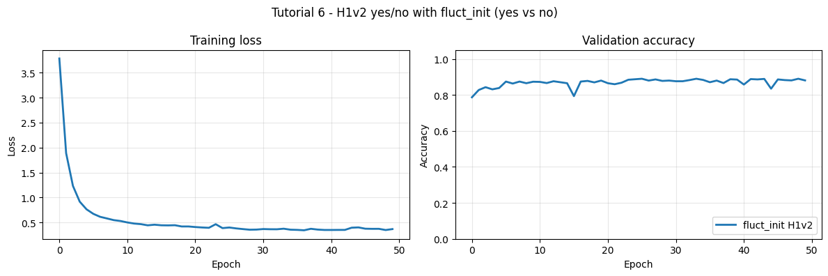
plot_histories(
{"fluct_init H1v2": history},
title=f"Tutorial 6 - H1v2 yes/no with fluct_init ({WORD_1} vs {WORD_2})",
)
print(f"\nBest validation accuracy: {best_acc:.1%}")
Running fluct_init on the H1v2 network...
[frontend_firing_init] target_fr=15.0%  n_batches=4  epsilon=2.0%  n_filters=13  [H1V2]


/tmp/ipykernel_106896/3400057061.py:21: UserWarning: Frontend on chip uses 16 filters. Using a different amount of neurons 13 is allowed but not respecting the chip constraints.
  self.frontend = H1v2Frontend(


  neuron | w         fr(cont)  fr(quant)
  neuron  0 | w=0.1714  fr=0.150  →0.170  [OK  ]
  neuron  1 | w=0.1644  fr=0.150  →0.185  [OK  ]
  neuron  2 | w=0.1623  fr=0.150  →0.189  [OK  ]
  neuron  3 | w=0.1637  fr=0.150  →0.186  [OK  ]
  neuron  4 | w=0.1633  fr=0.150  →0.185  [OK  ]
  neuron  5 | w=0.1631  fr=0.150  →0.185  [OK  ]
  neuron  6 | w=0.1684  fr=0.150  →0.177  [OK  ]
  neuron  7 | w=0.1739  fr=0.150  →0.167  [OK  ]
  neuron  8 | w=0.1786  fr=0.150  →0.159  [OK  ]
  neuron  9 | w=0.1830  fr=0.150  →0.152  [OK  ]
  neuron 10 | w=0.1871  fr=0.150  →0.146  [OK  ]
  neuron 11 | w=0.1878  fr=0.150  →0.145  [OK  ]
  neuron 12 | w=0.1882  fr=0.150  →0.145  [OK  ]
[frontend_firing_init] done.
[fluct_init] ξ=3.0  α=1.0  dt=8.0ms  (stacked, adaptive µ)  [H1V2]
  Frontend stage skipped — nu_out=56.7Hz used as nu_in for layer 1
  Layer 1 | ν_in=56.7Hz  µ_W=0.1922  σ_FF=0.2929  µ_U=0.099
           → nu_2 = 23.6 Hz


/opt/conda/envs/PyTorch/lib/python3.10/site-packages/IPython/core/interactiveshell.py:3336: UserWarning: fluct_init layer 2: 1/2 neurons are dead after init. The fluctuation-driven regime (σ_FF > 0) requires µ_W ≤ 0.1639, but avoiding dead neurons needs µ_W > 0.0205. Consider a smaller ξ, lower α, or more input neurons (n_F=64).
  has_raised = await self.run_ast_nodes(code_ast.body, cell_name,


  Layer 2 | ν_in=23.6Hz  µ_W=0.0226  σ_FF=0.3267  µ_U=0.024
[fluct_init] done.
=== H1v2 yes/no with fluct_init ===
epoch 01 | loss=3.7857 | train=71.0% | val=78.7%
epoch 05 | loss=0.7621 | train=85.1% | val=83.8%
epoch 10 | loss=0.5276 | train=85.9% | val=87.3%
epoch 15 | loss=0.4540 | train=86.9% | val=86.5%
epoch 20 | loss=0.4184 | train=87.3% | val=88.0%
epoch 25 | loss=0.3854 | train=87.2% | val=88.7%
epoch 30 | loss=0.3558 | train=88.6% | val=88.0%
epoch 35 | loss=0.3537 | train=88.6% | val=88.3%
epoch 40 | loss=0.3481 | train=88.7% | val=88.5%
epoch 45 | loss=0.3994 | train=87.6% | val=83.5%
epoch 50 | loss=0.3657 | train=89.0% | val=88.1%
Best validation accuracy: 89.0%
Best validation accuracy: 89.0%
6. Chip consumption calculation
Below we show how to estimate the chip consumption of this network over the dataset.
from nwavesdk.metrics import get_chip_consumption
# Run inference and collect spike data for power analysis
model.eval()
all_spk_frontend = []
all_spk_hidden   = []
all_spk_output   = []

with torch.no_grad():
    for x, y, fn in val_loader:
        x = x.to(device)
        spk_frontend, spk_hidden, spk_output = model(x)
        all_spk_frontend.append(spk_frontend)
        all_spk_hidden.append(spk_hidden)
        all_spk_output.append(spk_output)

all_spk_frontend = torch.cat(all_spk_frontend, dim=0)
all_spk_hidden = torch.cat(all_spk_hidden, dim=0)
all_spk_output = torch.cat(all_spk_output, dim=0)

spks = [all_spk_hidden, all_spk_output]

total_power = get_chip_consumption(model, spks, dt=8e-3)

n_timesteps = all_spk_hidden.shape[1]
energy_per_inference = total_power * n_timesteps * 8e-3

print("="*50)
print(f"HARDWARE POWER CONSUMPTION ({WORD_1} vs {WORD_2})")
print("="*50)
print(f"Total power:           {total_power*1e6:.3f} µW")
print(f"Energy per inference:  {energy_per_inference*1e9:.3f} nJ")
print(f"\nSpike rates:")
print(f"  Hidden layer: {all_spk_hidden.mean().item()*100:.1f}%")
print(f"  Output layer: {all_spk_output.mean().item()*100:.1f}%")
==================================================
HARDWARE POWER CONSUMPTION (yes vs no)
==================================================
Total power:           0.011 µW
Energy per inference:  11.266 nJ

Spike rates:
  Hidden layer: 33.0%
  Output layer: 15.6%


/tmp/ipykernel_106896/3821984310.py:21: UserWarning: Frontend power consumption is not supported yet. Skipping the initial Frontend -> Layer stage in power estimation.
  total_power = get_chip_consumption(model, spks, dt=8e-3)
7. Saving & loading models
Being NWAVE build upon torch, you can save and load models as plain torch's models.
torch.save(model, "h1v2_model_yesno.pt")
loaded = torch.load("h1v2_model_yesno.pt", map_location=device, weights_only=False)

model_to_load = loaded.to(device)
val_acc = evaluate(model_to_load, val_loader)
val_acc
0.8897058823529411
8. Summary
Tutorial 6 trains the same yes/no classifier as Tutorial 5 on the H1v2 chip. The key differences from the H1v1 path are:
| H1v1 (Tutorial 5) | H1v2 (Tutorial 6) | |
|---|---|---|
| Weight range | [-0.9, 0.9] |
[-1.66, 1.66] |
| Quantization bits | 5 | 6 |
| Frontend tau | 10 ms | 32 ms |
| fluct_init ξ target | — | 3.0 (higher to stay in range) |
| Core learning rate | 1e-3 | 3e-4 |
The initialization pipeline and hardware-aware loss stack are otherwise identical. For empirical parameter guidance see the official documentation.
Tutorial 7 extends H1v2 to recurrent (RC) networks for temporal pattern generation.