NWAVE Tutorial 2: H1v2 Model
This tutorial explores the H1v2 neuromorphic hardware model, comparing its dynamics against the software LIF baseline established in Tutorial 1 and the H1v2 neuromorphic hardware model.
By the end of this tutorial you will have:
- Observed how H1v2 membrane and spiking dynamics differ from LIF under identical inputs
- Understood which parameters are hardware-fixed and which remain configurable
- Seen how fabrication variability (
ileak_mismatch) spreads neuron responses - Applied
SignAnnealingto enforce the H1v2 block-of-5 sign constraint during training
1. Setup
import random
import numpy as np
import torch
import torch.nn as nn
import matplotlib.pyplot as plt

from nwavesdk.layers import (
    LIFSynapse,
    LIFLayer,
    H1v1Synapse,
    H1v1Layer,
    H1v2Synapse,
    H1v2Layer,
    prepare_net,
)

# Reproducibility
torch.manual_seed(7)
np.random.seed(7)
random.seed(7)
nwavesdk version: 1.0.0a0+cu


/opt/conda/envs/PyTorch/lib/python3.10/site-packages/tqdm/auto.py:21: TqdmWarning: IProgress not found. Please update jupyter and ipywidgets. See https://ipywidgets.readthedocs.io/en/stable/user_install.html
  from .autonotebook import tqdm as notebook_tqdm
2026-04-28 10:14:32,516 INFO util.py:154 -- Missing packages: ['ipywidgets']. Run `pip install -U ipywidgets`, then restart the notebook server for rich notebook output.
2026-04-28 10:14:32,765 INFO util.py:154 -- Missing packages: ['ipywidgets']. Run `pip install -U ipywidgets`, then restart the notebook server for rich notebook output.
2. LIF vs H1v2: What Is Configurable?
| Feature | LIFLayer / LIFSynapse |
H1v2Layer / H1v2Synapse |
|---|---|---|
| Threshold | User-set per layer; learn_thresholds=True supported |
Hardware-fixed; no constructor argument |
| Reset rule | "zero" / "subtraction" / "none" |
Fixed (subtraction + non-negative clamp) |
| Tau | Any float; learn_taus=True supported |
Snaps to hardware profiles |
| Weight range | Unbounded | [-1.66, 1.66] |
| Synapse mismatch (stddev) | Not modelled | Not available — H1v2 mismatch is layer-only (ileak_mismatch) |
The code cells below demonstrate each constraint directly.
- No synapse stddev —
H1v1Synapseaccepts astddevparameter for per-weight Gaussian noise;H1v2Synapsedoes not. - Wider weight range — H1v1 uses
[-0.9, 0.9]; H1v2 uses[-1.66, 1.66]. - Lower synaptic gain — each unit of synaptic weight produces a smaller membrane increment in H1v2 than in H1v1, due to the hardware's linear current model (
dV = fo · w). This is why H1v2 networks need larger weights or more inputs to drive neurons to threshold.
# LIF accepts explicit thresholds
lif_ok = LIFLayer(
    n_neurons=1,
    taus=20e-3,
    thresholds=0.25,
    reset_mechanism="subtraction",
    dt=1e-3,
    device="cpu",
)
print("LIF threshold set to:", float(lif_ok.thresholds.item()))

# H1v2: trying to set thresholds should fail at API level
try:
    _ = H1v2Layer(n_neurons=1, taus=20e-3, dt=1e-3, thresholds=0.25)
except TypeError as e:
    print("H1v2Layer rejects custom `thresholds`:")
    print("  ", e)

# H1v2 synapse: no stddev mismatch argument in H1v2 API
try:
    _ = H1v2Synapse(nb_inputs=1, nb_outputs=1, stddev=0.02)
except TypeError as e:
    print("H1v2Synapse rejects `stddev` in constructor:")
    print("  ", e)
LIF threshold set to: 0.25
H1v2Layer rejects custom `thresholds`:
   __init__() got an unexpected keyword argument 'thresholds'
H1v2Synapse rejects `stddev` in constructor:
   __init__() got an unexpected keyword argument 'stddev'
3. Helper Functions
def make_spike_train(T=80, spike_times=(10,)):
    x = torch.zeros(1, T, 1, dtype=torch.float32)
    for t in spike_times:
        x[:, t, 0] = 1.0
    return x


def simulate_stack(syn, layer, x):
    """Run a single synapse->layer stack over time."""
    # Prepare/reset all internal runtime buffers
    bundle = nn.ModuleList([syn, layer])
    prepare_net(bundle)

    cur_trace, spk_trace, mem_trace = [], [], []

    for t in range(x.shape[1]):
        cur = syn(x[:, t, :])
        spk, mem = layer(cur)

        cur_trace.append(cur.detach().cpu())
        spk_trace.append(spk.detach().cpu())
        mem_trace.append(mem.detach().cpu())

    return (
        torch.stack(cur_trace, dim=1),
        torch.stack(spk_trace, dim=1),
        torch.stack(mem_trace, dim=1),
    )  # all tensors [B, T, N]
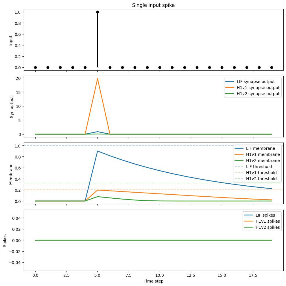
4. Single Input Spike at Parity of Input and Tau
All models receive the same spike train, nominal tau, and synapse weight. Despite identical inputs, responses diverge because:
- Membrane jump: H1v2 synaptic output is hardware-mapped with a lower gain constant than both LIF and H1v1. The same nominal weight produces a smaller membrane increment in H1v2 than in H1v1, and a smaller increment still compared to LIF (where weight directly equals membrane jump).
- Threshold: H1v2's hardware threshold (
_vt) is higher than H1v1's, requiring more accumulated charge to fire. - Decay law: both H1v1 and H1v2 use linear decay (not exponential)
H1v2 therefore needs more input spikes to reach threshold than H1v1 under the same nominal weight, and more still than LIF.
dt = 1e-3
tau = 10e-3
lif_threshold = 1.0

x = make_spike_train(T=20, spike_times=(5,))

# LIF stack
lif_syn = LIFSynapse(1, 1, device="cpu")
lif_layer = LIFLayer(
    n_neurons=1,
    taus=tau,
    thresholds=1,
    reset_mechanism="subtraction",
    dt=dt,
    device="cpu",
)

# H1v1 stack
h1_syn = H1v1Synapse(1, 1, device="cpu", lif_threshold=lif_threshold)
h1_layer = H1v1Layer(
    n_neurons=1,
    taus=tau,
    dt=dt,
    ileak_mismatch=False,
    device="cpu",
)


# H1v2 stack
h2_syn = H1v2Synapse(1, 1, device="cpu", lif_threshold=lif_threshold)
h2_layer = H1v2Layer(
    n_neurons=1,
    taus=tau,
    dt=dt,
    ileak_mismatch=False,
    device="cpu",
)

# Force same visible initialization for both synapses
with torch.no_grad():
    lif_syn.weight.fill_(0.9)
    h1_syn.weight.fill_(0.9)
    h2_syn.weight.fill_(0.9)

cur_lif, spk_lif, mem_lif = simulate_stack(lif_syn, lif_layer, x)
cur_hwv1, spk_hwv1, mem_hwv1 = simulate_stack(h1_syn, h1_layer, x)
cur_hwv2, spk_hwv2, mem_hwv2 = simulate_stack(h2_syn, h2_layer, x)

print(
    f"Peak synaptic output: LIF={cur_lif.max():.4f}, H1v1={cur_hwv1.max():.4f}, H1v2={cur_hwv2.max():.4f}"
)
print(
    f"Total spikes:         LIF={spk_lif.sum():.0f}, H1v1={spk_hwv1.sum():.0f}, H1v2={spk_hwv2.sum():.0f}"
)
print(
    f"Peak membrane:        LIF={mem_lif.max():.4f}, H1v1={mem_hwv1.max():.4f}, H1v2={mem_hwv2.max():.4f}"
)


def plot_lif_vs_h2(
    x,
    cur_lif,
    spk_lif,
    mem_lif,
    cur_hwv1,
    spk_hwv1,
    mem_hwv1,
    cur_hwv2,
    spk_hwv2,
    mem_hwv2,
):
    (
        cur_lif,
        spk_lif,
        mem_lif,
        cur_hwv1,
        spk_hwv1,
        mem_hwv1,
        cur_hwv2,
        spk_hwv2,
        mem_hwv2,
    ) = (
        cur_lif[0, :, 0],
        spk_lif[0, :, 0],
        mem_lif[0, :, 0],
        cur_hwv1[0, :, 0],
        spk_hwv1[0, :, 0],
        mem_hwv1[0, :, 0],
        cur_hwv2[0, :, 0],
        spk_hwv2[0, :, 0],
        mem_hwv2[0, :, 0],
    )  # let's look at the 0-th batch and the  0-th neuron
    t = np.arange(x.shape[1])
    fig, ax = plt.subplots(4, 1, figsize=(10, 10), sharex=True)

    ax[0].stem(t, x[0, :, 0].numpy(), basefmt=" ", linefmt="k-", markerfmt="ko")
    ax[0].set_ylabel("Input")
    ax[0].set_title("Single input spike")

    ax[1].plot(t, cur_lif, label="LIF synapse output", lw=2)
    ax[1].plot(t, cur_hwv1, label="H1v1 synapse output", lw=2)
    ax[1].plot(t, cur_hwv2, label="H1v2 synapse output", lw=2)
    ax[1].set_ylabel("Syn output")
    ax[1].legend()

    ax[2].plot(t, mem_lif, label="LIF membrane", lw=2)
    ax[2].plot(t, mem_hwv1, label="H1v1 membrane", lw=2)
    ax[2].plot(t, mem_hwv2, label="H1v2 membrane", lw=2)
    ax[2].axhline(
        lif_threshold, ls="--", color="tab:blue", alpha=0.3, label="LIF threshold"
    )
    ax[2].axhline(0.204, ls="--", color="tab:orange", alpha=0.3, label="H1v1 threshold")
    ax[2].axhline(0.322, ls="--", color="tab:green", alpha=0.3, label="H1v2 threshold")
    ax[2].set_ylabel("Membrane")
    ax[2].legend()

    ax[3].plot(t, spk_lif, label="LIF spikes", lw=2)
    ax[3].plot(t, spk_hwv1, label="H1v1 spikes", lw=2)
    ax[3].plot(t, spk_hwv2, label="H1v2 spikes", lw=2)
    ax[3].set_ylabel("Spikes")
    ax[3].set_xlabel("Time step")
    ax[3].legend()

    plt.tight_layout()
    plt.show()


plot_lif_vs_h2(
    x,
    cur_lif,
    spk_lif,
    mem_lif,
    cur_hwv1,
    spk_hwv1,
    mem_hwv1,
    cur_hwv2,
    spk_hwv2,
    mem_hwv2,
)
Peak synaptic output: LIF=0.9000, H1v1=19.7304, H1v2=0.0786
Total spikes:         LIF=0, H1v1=0, H1v2=0
Peak membrane:        LIF=0.9000, H1v1=0.1973, H1v2=0.0786
# Numeric comparison: threshold and synaptic gain for H1v1 vs H1v2
h1_ref = H1v1Layer(n_neurons=1, taus=tau, dt=dt, device="cpu")
h2_ref = H1v2Layer(n_neurons=1, taus=tau, dt=dt, device="cpu")
prepare_net(h1_ref)
prepare_net(h2_ref)

# Set weights before prepare_net, as this function call is needed before inference/training but always after parameter changes
h1_syn_ref = H1v1Synapse(1, 1, device="cpu")
h2_syn_ref = H1v2Synapse(1, 1, device="cpu")
with torch.no_grad():
    h1_syn_ref.weight[0] = 1
    h2_syn_ref.weight[0] = 1

prepare_net(h1_syn_ref)
prepare_net(h2_syn_ref)

x_one = torch.ones(1, 1)
h1_cur = h1_syn_ref(x_one).item()
h2_cur = h2_syn_ref(x_one).item()

print("--- Hardware threshold (_vt) ---")
print(f"  H1v1: {float(h1_ref._vt.mean()):.4f} V")
print(f"  H1v2: {float(h2_ref._vt.mean()):.4f} V")
print()
print("--- Synaptic current for weight=1, one spike ---")
print(f"  LIF : 1.0000  (weight maps directly to membrane jump)")
print(f"  H1v1: {h1_cur:.4f}")
print(f"  H1v2: {h2_cur:.4f}")
print()
print(f"Spikes needed to reach threshold (weight=1, no decay):")
print(f"  LIF : {1.0 / 1.0:.5f}")
print(f"  H1v1: {float(h1_ref._vt.mean()) / h1_cur:.5f}")
print(f"  H1v2: {float(h2_ref._vt.mean()) / h2_cur:.5f}")
--- Hardware threshold (_vt) ---
  H1v1: 0.2040 V
  H1v2: 0.3226 V

--- Synaptic current for weight=1, one spike ---
  LIF : 1.0000  (weight maps directly to membrane jump)
  H1v1: 21.3811
  H1v2: 0.0873

Spikes needed to reach threshold (weight=1, no decay):
  LIF : 1.00000
  H1v1: 0.00954
  H1v2: 3.69324
Interpretation
The three models behave differently even at identical weight and nominal tau:
| LIF | H1v1 | H1v2 | |
|---|---|---|---|
| Membrane jump per spike (weight=1) | 1.0 (exact) | hardware-mapped, < 1 | hardware-mapped, < H1v1 |
| Threshold | User-set (1.0 here) | ~0.2 V (chip-level) | higher than H1v1 (chip-level) |
| Spikes to threshold (weight=1) | fewest | more than LIF | more than H1v1 |
H1v2's lower synaptic gain is networks often need more input channels or higher weights than their H1v1 equivalents.
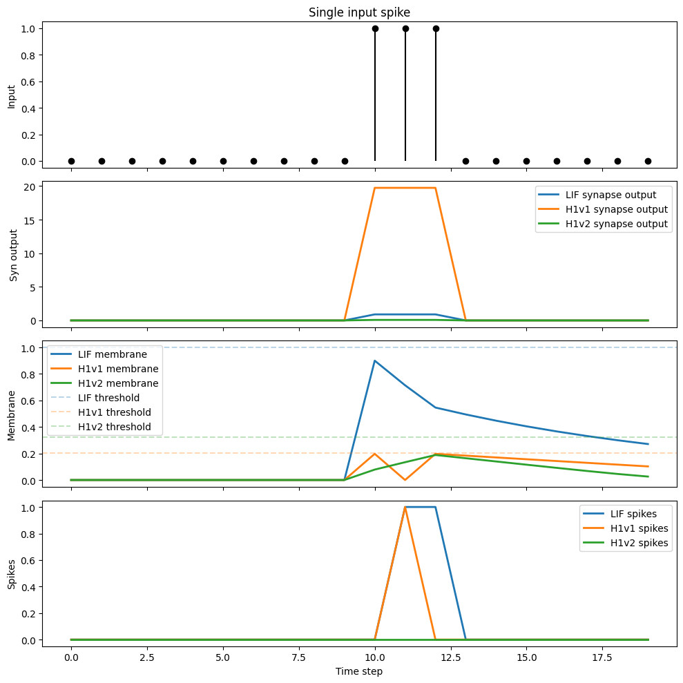
The next experiment increases the number of input spikes to drive the H1v2 model to threshold.
x = make_spike_train(T=20, spike_times=(10, 11, 12))


cur_lif, spk_lif, mem_lif = simulate_stack(lif_syn, lif_layer, x)
cur_hwv1, spk_hwv1, mem_hwv1 = simulate_stack(h1_syn, h1_layer, x)
cur_hwv2, spk_hwv2, mem_hwv2 = simulate_stack(h2_syn, h2_layer, x)

plot_lif_vs_h2(
    x,
    cur_lif,
    spk_lif,
    mem_lif,
    cur_hwv1,
    spk_hwv1,
    mem_hwv1,
    cur_hwv2,
    spk_hwv2,
    mem_hwv2,
)
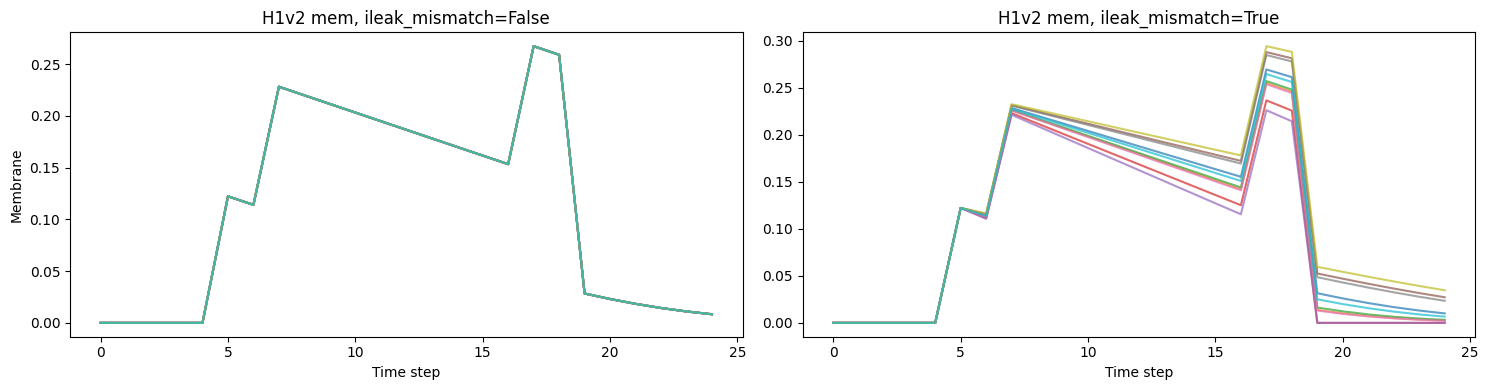
5. H1v2 Non-Idealities: Threshold and Leak Variability
H1v2 mismatch is layer-only: ileak_mismatch=True adds per-neuron variability in the leak current, spreading membrane trajectories across the population. Unlike H1v1, H1v2 has no stddev parameter on the synapse — weight-level noise is absent.
We compare ileak_mismatch=False vs ileak_mismatch=True on a population of 40 neurons with identical weights:
- Without mismatch, neurons overlap in response.
- With mismatch, membrane trajectories and spike counts diverge.
def run_h2_population(ileak_mismatch, n_neurons=40, tau=20e-3, w=1.4, seed=7):
    torch.manual_seed(seed)

    syn = H1v2Synapse(1, n_neurons, device="cpu", lif_threshold=1.0)
    layer = H1v2Layer(
        n_neurons=n_neurons,
        taus=tau,
        dt=1e-3,
        ileak_mismatch=ileak_mismatch,
        device="cpu",
    )

    with torch.no_grad():
        syn.weight.fill_(w)

    _, spk_hw, mem_hw = simulate_stack(syn, layer, x_multi)
    return mem_hw, spk_hw


x_multi = make_spike_train(T=25, spike_times=(5, 7, 17, 19))

mem_nom, spk_nom = run_h2_population(ileak_mismatch=False)
mem_mis, spk_mis = run_h2_population(ileak_mismatch=True)

spk_count_nom = (spk_nom > 0.5).sum(axis=0)
spk_count_mis = (spk_mis > 0.5).sum(axis=0)

fig, ax = plt.subplots(1, 2, figsize=(15, 4))

for n in range(10):
    ax[0].plot(
        mem_nom[0, :, n], alpha=0.7, lw=1.5
    )  # plot neurons over the 0-th batch input
ax[0].set_title("H1v2 mem, ileak_mismatch=False")
ax[0].set_xlabel("Time step")
ax[0].set_ylabel("Membrane")

for n in range(10):
    ax[1].plot(
        mem_mis[0, :, n], alpha=0.7, lw=1.5
    )  # plot neurons over the 0-th batch input
ax[1].set_title("H1v2 mem, ileak_mismatch=True")
ax[1].set_xlabel("Time step")


plt.tight_layout()
plt.show()
6. Tau Request vs Effective Tau
With the same user-requested tau, LIF keeps that value directly, while H1v2 may snap tau to supported hardware profiles.
tau_requested = 17e-3

lif_tau = LIFLayer(
    n_neurons=1,
    taus=tau_requested,
    thresholds=0.3,
    reset_mechanism="subtraction",
    dt=1e-3,
    device="cpu",
)

h2_tau = H1v2Layer(
    n_neurons=1,
    taus=tau_requested,
    dt=1e-3,
    ileak_mismatch=False,
    device="cpu",
)

print(f"Requested tau: {tau_requested * 1e3:.3f} ms")
print(f"LIF effective tau: {float(lif_tau.taus.item()) * 1e3:.3f} ms")
print(f"H1v2 effective tau:  {float(h2_tau.taus.item()) * 1e3:.3f} ms")
Requested tau: 17.000 ms
LIF effective tau: 17.000 ms
H1v2 effective tau:  13.820 ms
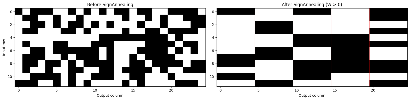
7. Weight constraints and block-of-5 sign topology
The sign-topology constraint is shared with H1v1 (see Tutorial 1 Section 4f). The mechanism is identical — the analog routing fabric groups every 5 inputs per output neuron into a block, and all weights in a block must share the same sign. The key difference is the weight range:
| H1v1 | H1v2 | |
|---|---|---|
| Weight range | [-0.9, 0.9] |
[-1.66, 1.66] |
| Sign topology | Block of 5 | Block of 5 |
SignAnnealing enforces the sign constraint during training by progressively hardening block-level sign agreement while keeping gradient flow through magnitudes. The demonstrative training run below uses H1v2 weights.
from nwavesdk.optim import SignAnnealing


class ToyH2Net(nn.Module):
    def __init__(self, n_in, n_out=2):
        super().__init__()
        self.syn = H1v2Synapse(
            n_in,
            n_out,
        )

    def forward(self, x):
        T = x.shape[1]
        trace = []
        prepare_net(self)

        for t in range(T):
            cur_hidden = self.syn(x[:, t, :])
            trace.append(cur_hidden)

        return torch.stack(trace, dim=1)
# Fake dataset (random inputs/targets): this is only to demonstrate the topology behavior
n_in, n_out = 12, 25
x_fake = torch.randn(1, 128, n_in)
y_fake = torch.randn(1, 128, n_out)

net = ToyH2Net(n_in, n_out)

W_unconstrained = net.syn.weight.detach().clone()

epochs = 10
sign_annealer = SignAnnealing(net, total_epochs=epochs, alpha_start=0.5, alpha_end=12.0)
optimizer = torch.optim.Adam(net.parameters(), lr=5e-2)

loss_hist = []

for epoch in range(1, epochs + 1):
    sign_annealer.step(net, epoch)

    pred = net(x_fake)
    loss = torch.mean((pred - y_fake) ** 2)

    optimizer.zero_grad()
    loss.backward()
    optimizer.step()

    with torch.no_grad():
        loss_hist.append(float(loss.item()))

W_final = net.syn.weight.detach().cpu()
fig, ax = plt.subplots(1, 2, figsize=(16, 4))

ax[0].imshow((W_unconstrained.cpu().numpy() > 0), aspect="auto", cmap="gray_r")
ax[0].set_title("Before SignAnnealing")
ax[0].set_xlabel("Output column")
ax[0].set_ylabel("Input row")

ax[1].imshow((W_final.numpy() > 0), aspect="auto", cmap="gray_r")
ax[1].set_title("After SignAnnealing (W > 0)")
ax[1].set_xlabel("Output column")

for c in range(5, n_out, 5):
    ax[1].axvline(c - 0.5, color="red", lw=0.8, alpha=0.6)

plt.tight_layout()
plt.show()
8. Summary
| Parameter / Feature | LIFLayer |
H1v2Layer |
|---|---|---|
| Tau (τ) | Any float; learn_taus=True stores _d_taus as nn.Parameter |
Set at init → _Ileak; not a gradient-learnable parameter |
| Threshold (θ) | Per-layer; learn_thresholds=True makes it learnable |
Fixed chip-wide; same for all layers; not learnable |
| Reset mechanism | subtraction / zero / none |
Fixed (subtraction + non-negative clamp) |
| Membrane polarity | Can go negative | Always >= 0 (hardware clamp) |
| Weight range | Unbounded | Bounded to [-1.66, 1.66] (H1v1 uses [-0.9, 0.9]) |
| Sign topology | No constraint | Groups of 5 weights must share sign (shared with H1v1) |
| Synapse mismatch (stddev) | Not modelled | Not available — H1v1Synapse supports stddev; H1v2Synapse does not |
| Layer variability | Not modelled | ileak_mismatch=True (also present in H1v1) |
| Primary use case | Research, prototyping | Hardware deployment on Neuronova H1v2 |
Next Steps
Tutorial 3 covers CPU/GPU execution: how to port H1v1 and H1v2 networks to GPU, verify numerical equivalence, and benchmark inference and training throughput.