NWAVE Tutorial 4: Audio Classification on H1v1 Hardware Model
This notebook shows how to build, train, and evaluate a network built on H1v1 for the Google Speech Commands yes/no task.
This is the first tutorial to bridge the gap between simulation and real hardware. By the end you will have trained three variants of the same network, each progressively more aware of H1v1 hardware realities:
- Plain H1v1 — FP32 weights, no hardware constraints (accuracy ceiling)
- Hardware-aware H1v1 — quantization + routing and range constraints enforced during training (chip-deployable)
- Mismatch-aware H1v1 — adds simulation of analog device variability (most realistic, best transfer to physical hardware)
1. Setup and Imports
import os
import shutil
import time

import matplotlib.pyplot as plt
import numpy as np
import scipy.io.wavfile as wavfile
import torch
import torch.nn as nn
from torchaudio.datasets import SPEECHCOMMANDS

from nwavesdk import NWaveDataGen, NWaveDataloaderConfig
from nwavesdk.layers import H1v1Frontend, H1v1Synapse, H1v1Layer, prepare_net
from nwavesdk.loss import (
    topology_loss,
    weight_magnitude_loss,
    firing_rate_target_mse_loss,
)
from nwavesdk.metrics import accuracy
from nwavesdk.surrogate import fast_sigmoid


device = torch.device("cuda" if torch.cuda.is_available() else "cpu")
device_flag = "gpu" if device.type == "cuda" else "cpu"

torch.manual_seed(42)
np.random.seed(42)

print(f"Device: {device}")
nwavesdk version: 1.0.0a0+rocm


/opt/conda/envs/PyTorch/lib/python3.10/site-packages/tqdm/auto.py:21: TqdmWarning: IProgress not found. Please update jupyter and ipywidgets. See https://ipywidgets.readthedocs.io/en/stable/user_install.html
  from .autonotebook import tqdm as notebook_tqdm
2026-04-27 16:50:09,842 INFO util.py:154 -- Missing packages: ['ipywidgets']. Run `pip install -U ipywidgets`, then restart the notebook server for rich notebook output.
2026-04-27 16:50:09,963 INFO util.py:154 -- Missing packages: ['ipywidgets']. Run `pip install -U ipywidgets`, then restart the notebook server for rich notebook output.


Device: cuda
2. Dataset and Preprocessing
We use the Google Speech Commands dataset, a popular benchmark for keyword spotting.
Available words: yes, no, up, down, left, right, on, off, stop, go, and more.
Task: Binary classification between 2 selected words.
Configuration: You can change WORD_1 and WORD_2 below to use any pair of words.
# ============================================
# CONFIGURATION: Choose your 2 words
# ============================================
# Available words in Speech Commands v0.02:
# yes, no, up, down, left, right, on, off, stop, go,
# zero, one, two, three, four, five, six, seven, eight, nine,
# bed, bird, cat, dog, happy, house, marvin, sheila, tree, wow

WORD_1 = "yes"  # Class 0
WORD_2 = "no"  # Class 1

# Audio parameters
SAMPLE_RATE = 16000  # Speech Commands native sample rate
RECORDING_DURATION_S = 1.0  # Each clip is 1 second

print(f"Training binary classifier: '{WORD_1}' (class 0) vs '{WORD_2}' (class 1)")
Training binary classifier: 'yes' (class 0) vs 'no' (class 1)
from torchaudio.datasets import SPEECHCOMMANDS

# Download Speech Commands dataset
os.makedirs("data", exist_ok=True)


class SubsetSpeechCommands(SPEECHCOMMANDS):
    """Speech Commands dataset filtered to specific words."""

    def __init__(self, root, subset, words, download=True):
        super().__init__(root, download=download, subset=subset)
        self.words = words
        # Filter to only include specified words
        self._walker = [
            item
            for item in self._walker
            if os.path.basename(os.path.dirname(item)) in words
        ]


# Load training and validation subsets
print(f"Downloading Speech Commands dataset (this may take a few minutes)...")
train_dataset = SubsetSpeechCommands("data", subset="training", words=[WORD_1, WORD_2])
val_dataset = SubsetSpeechCommands("data", subset="validation", words=[WORD_1, WORD_2])

print(f"\nDataset loaded:")
print(f"  Training samples: {len(train_dataset)}")
print(f"  Validation samples: {len(val_dataset)}")
Downloading Speech Commands dataset (this may take a few minutes)...

Dataset loaded:
  Training samples: 6358
  Validation samples: 803
import scipy.io.wavfile as wavfile

# Prepare data directory structure for NWaveDataGen
# NWaveDataGen expects: data_parent/class_name/*.wav

target_dir = "data_for_nwave_commands"
word1_dir = os.path.join(target_dir, WORD_1)
word2_dir = os.path.join(target_dir, WORD_2)

# Clean and create directories
if os.path.exists(target_dir):
    shutil.rmtree(target_dir)
os.makedirs(word1_dir, exist_ok=True)
os.makedirs(word2_dir, exist_ok=True)


def save_dataset_to_folders(dataset, word1_dir, word2_dir, word1, word2, prefix=""):
    """Save dataset samples to class folders as WAV files."""
    counts = {word1: 0, word2: 0}

    for i, (waveform, sample_rate, label, speaker_id, utterance_num) in enumerate(
        dataset
    ):
        # Determine output directory based on label
        if label == word1:
            out_dir = word1_dir
        elif label == word2:
            out_dir = word2_dir
        else:
            continue

        # Convert to numpy and ensure correct format
        audio = waveform.squeeze().numpy()

        # Pad or trim to exactly 1 second
        target_length = sample_rate  # 1 second
        if len(audio) < target_length:
            audio = np.pad(audio, (0, target_length - len(audio)))
        else:
            audio = audio[:target_length]

        # Convert to int16 for WAV file (scipy.io.wavfile format)
        audio_int16 = (audio * 32767).astype(np.int16)

        # Save file
        filename = f"{prefix}{label}_{speaker_id}_{utterance_num}_{i}.wav"
        filepath = os.path.join(out_dir, filename)
        wavfile.write(filepath, sample_rate, audio_int16)
        counts[label] += 1

    return counts


# Save training data
print("Preparing training data...")
train_counts = save_dataset_to_folders(
    train_dataset, word1_dir, word2_dir, WORD_1, WORD_2, prefix="train_"
)

# Save validation data
print("Preparing validation data...")
val_counts = save_dataset_to_folders(
    val_dataset, word1_dir, word2_dir, WORD_1, WORD_2, prefix="val_"
)

print(f"\nData prepared in '{target_dir}':")
print(f"  {WORD_1}/: {train_counts[WORD_1] + val_counts[WORD_1]} files")
print(f"  {WORD_2}/: {train_counts[WORD_2] + val_counts[WORD_2]} files")
Preparing training data...
Preparing validation data...

Data prepared in 'data_for_nwave_commands':
  yes/: 3625 files
  no/: 3536 files
NWaveDataGen applies the H1v1 chip's own filterbank to produce chip-realistic input — the same 16-channel frequency decomposition the physical frontend performs. Training on this output ensures the model never sees a feature the hardware cannot produce.
We use sim_time_s=8e-3 to set the simulation timestep. The simulation timestep will be then used as a parameter for simulating the layers in the next code snippets. This is not a hardware clock (H1v1 is fully analog). A larger timestep means fewer time steps for the same audio clip, which speeds up simulation at the cost of temporal resolution. For this 1-second clip at 8 ms: 1 s ÷ 8 ms = 125 timesteps.
from nwavesdk import NWaveDataGen, NWaveDataloaderConfig

# Creating a dataloader config
data_config = NWaveDataloaderConfig(
    batch_size=16,
    val_split=0.15,
    test_split=0.0,
    random_state=123,
    num_workers=4,
    shuffle_train=True,
)

# Create data generator with hardware filterbank
dm = NWaveDataGen(
    data_parent=target_dir,
    sample_rate=SAMPLE_RATE,
    recording_duration_s=RECORDING_DURATION_S,
    sim_time_s=8e-3,  # 8ms time bins
    dataloader_config=data_config,
    task="classification",
    return_filename=True,
)

loaders = dm.dataloaders()
train_loader = loaders["train"]
val_loader = loaders["val"]

# Get number of filter channels from first batch (based on the Nyquist freq)
x, y, fn = next(iter(train_loader))
N_CHANNELS = x.shape[2]
print(f"\nInput shape: {x.shape} (batch, timesteps, channels)")
print(f"Number of filter channels: {N_CHANNELS}")
print(
    f"\nDataset split: {len(train_loader.dataset)} train, {len(val_loader.dataset)} validation"
)
2026-04-27 16:50:26,933 - root - WARNING - Using 13 valid freqs out of 16 for sr=16000Hz (Nyquist=8000.0Hz).
Classes (loading wavs): 100%|██████████| 2/2 [00:03<00:00,  1.69s/it]
Filtering no: 100%|██████████| 3536/3536 [00:00<00:00, 4613.52it/s]
Filtering yes: 100%|██████████| 3625/3625 [00:00<00:00, 4229.85it/s]


Input shape: torch.Size([16, 125, 13]) (batch, timesteps, channels)
Number of filter channels: 13

Dataset split: 6087 train, 1074 validation
# # (Optional) Save/Load dataloader
torch.save(train_loader, "train_commands.pt")
torch.save(val_loader, "val_commands.pt")

train_loader = torch.load("train_commands.pt", weights_only=False)
val_loader = torch.load("val_commands.pt", weights_only=False)
3. H1v1 model definition
Input → H1v1Frontend → H1v1Layer → H1v1Synapse → H1v1Layer → H1v1Synapse → H1v1Layer
prepare_net(model) must be called once per batch before the forward pass. It resets internal layer states and prepares hardware-specific buffers — skipping it leaves the model in a stale state.
def dense_topology_penalty(model, lam):
    return topology_loss(model.syn_hidden, lam=lam) + topology_loss(
        model.syn_out, lam=lam
    )


class H1v1YesNoNet(nn.Module):
    """Frontend-first H1v1 classifier for yes/no keyword spotting."""

    def __init__(self, n_channels, hidden_size=64, num_classes=2, quantized=False):
        super().__init__()
        self.device_flag = device_flag
        slope = fast_sigmoid(slope=25.0)

        frontend_kwargs = {}
        dense_kwargs = {}
        if quantized:
            frontend_kwargs["quantization_bit"] = 5
            dense_kwargs["quantization_bit"] = 5

        # Plain keeps this FP32; quantized=True switches to the hardware-aware path.
        self.frontend = H1v1Frontend(
            nb_inputs=n_channels,
            device=self.device_flag,
            **frontend_kwargs,
        )
        self.frontend_layer = H1v1Layer(
            n_neurons=n_channels,
            taus=10e-3,
            dt=8e-3,
            spike_grad=slope,
            device=self.device_flag,
        )

        self.syn_hidden = H1v1Synapse(
            n_channels,
            hidden_size,
            device=self.device_flag,
            **dense_kwargs,
        )
        self.hidden = H1v1Layer(
            n_neurons=hidden_size,
            taus=64e-3,
            dt=8e-3,
            spike_grad=slope,
            device=self.device_flag,
        )

        self.syn_out = H1v1Synapse(
            hidden_size,
            num_classes,
            device=self.device_flag,
            **dense_kwargs,
        )
        self.out = H1v1Layer(
            n_neurons=num_classes,
            taus=64e-3,
            dt=8e-3,
            spike_grad=slope,
            device=self.device_flag,
        )

        self.frontend_stage = (self.frontend, self.frontend_layer)
        self.layer_pairs = [(self.syn_hidden, self.hidden), (self.syn_out, self.out)]

    def forward(self, x):
        prepare_net(self, collect_metrics=False)

        if self.device_flag == "gpu":
            cur0 = self.frontend(x)
            spk0, _ = self.frontend_layer(cur0)
            cur1 = self.syn_hidden(spk0)
            spk1, _ = self.hidden(cur1)
            cur2 = self.syn_out(spk1)
            spk2, _ = self.out(cur2)
            self.frontend_trace = spk0
            self.hidden_trace = spk1
            self.output_trace = spk2
            return spk2

        frontend_spk = []
        hidden_spk = []
        output_spk = []

        for t in range(x.shape[1]):
            cur0 = self.frontend(x[:, t, :])
            spk0, _ = self.frontend_layer(cur0)
            cur1 = self.syn_hidden(spk0)
            spk1, _ = self.hidden(cur1)
            cur2 = self.syn_out(spk1)
            spk2, _ = self.out(cur2)
            frontend_spk.append(spk0)
            hidden_spk.append(spk1)
            output_spk.append(spk2)

        self.frontend_trace = torch.stack(frontend_spk, dim=1)
        self.hidden_trace = torch.stack(hidden_spk, dim=1)
        self.output_trace = torch.stack(output_spk, dim=1)
        return self.output_trace
4. Training utilities
evaluate sums spikes over the time dimension and uses spike count as the confidence score for classification — the output neuron with the most spikes wins.
def evaluate(model, loader):
    model.eval()
    correct = 0.0
    total = 0
    with torch.no_grad():
        for specs, labels, _ in loader:
            specs = specs.to(device)
            labels = labels.to(device)
            spike_traces = model(specs)
            correct += accuracy(spike_traces, labels)
            total += 1
    return correct / max(total, 1)


def train_model(
    model,
    train_loader,
    val_loader,
    *,
    name,
    epochs=50,
    lr_frontend=1e-5,
    lr_core=1e-3,
    lam_topology=0.0,
    lam_fr=0.0,
    target_fr=0.15,
    limit=0.9,
):
    criterion = nn.CrossEntropyLoss()
    optimizer = torch.optim.Adam(
        [
            {
                "params": list(model.frontend.parameters())
                + list(model.frontend_layer.parameters()),
                "lr": lr_frontend,
            },
            {
                "params": list(model.syn_hidden.parameters())
                + list(model.hidden.parameters())
                + list(model.syn_out.parameters())
                + list(model.out.parameters()),
                "lr": lr_core,
            },
        ]
    )

    history = {"train_loss": [], "train_acc": [], "val_acc": []}
    best_acc = 0.0
    best_state = None

    print(f"\n=== {name} ===")
    for epoch in range(1, epochs + 1):
        model.train()
        running_loss = 0.0
        running_correct = 0
        running_total = 0

        for specs, labels, _ in train_loader:
            specs = specs.to(device)
            labels = labels.to(device)

            optimizer.zero_grad()
            spike_traces = model(specs)
            logits = spike_traces.sum(dim=1)

            loss_main = criterion(logits, labels)
            # Loss stack = topology_loss + weight_magnitude_loss + firing_rate_target_mse_loss.
            loss_topo = (
                dense_topology_penalty(model, lam_topology)
                if lam_topology
                else torch.zeros((), device=logits.device)
            )

            loss_mag = weight_magnitude_loss(model, limit=limit)
            loss_fr = (
                firing_rate_target_mse_loss(
                    spikes_list=[spike_traces],
                    offsets=[target_fr],
                    multipliers=[lam_fr],
                )
                if lam_fr
                else torch.zeros((), device=logits.device)
            )

            loss = loss_main + loss_topo + loss_mag + loss_fr
            loss.backward()
            # Gradient clipping is still useful with the regularizer stack, especially under mismatch.
            torch.nn.utils.clip_grad_norm_(model.parameters(), max_norm=0.5)
            optimizer.step()

            preds = logits.argmax(dim=1)
            running_correct += (preds == labels).sum().item()
            running_total += labels.size(0)
            running_loss += loss.item() * labels.size(0)

        train_acc = running_correct / max(running_total, 1)
        train_loss = running_loss / max(len(train_loader.dataset), 1)
        val_acc = evaluate(model, val_loader)

        history["train_loss"].append(train_loss)
        history["train_acc"].append(train_acc)
        history["val_acc"].append(val_acc)

        if val_acc >= best_acc:
            best_acc = val_acc
            best_state = {
                k: v.detach().cpu().clone() for k, v in model.state_dict().items()
            }

        if epoch == 1 or epoch % 5 == 0:
            print(
                f"epoch {epoch:02d} | loss={train_loss:.4f} | train={train_acc:.1%} | val={val_acc:.1%}"
            )

    if best_state is not None:
        model.load_state_dict(best_state)

    print(f"Best validation accuracy: {best_acc:.1%}")
    return history, best_acc


def plot_histories(histories, title):
    fig, axes = plt.subplots(1, 2, figsize=(12, 4))
    for label, history in histories.items():
        axes[0].plot(history["train_loss"], linewidth=2, label=label)
        axes[1].plot(history["val_acc"], linewidth=2, label=label)
    axes[0].set_title("Training loss")
    axes[0].set_xlabel("Epoch")
    axes[0].set_ylabel("Loss")
    axes[0].grid(True, alpha=0.3)
    axes[1].set_title("Validation accuracy")
    axes[1].set_xlabel("Epoch")
    axes[1].set_ylabel("Accuracy")
    axes[1].set_ylim(0.0, 1.05)
    axes[1].grid(True, alpha=0.3)
    axes[1].legend(loc="lower right")
    fig.suptitle(title)
    plt.tight_layout()
    plt.show()
5. Plain H1v1 training (no non-idealities)
FP32 weights, no quantization, no mismatch, no topology enforcement, just firing rate regularization to avoid dead/always-firing neurons and magnitude loss to avoid unnatural ranges of weights. This is the accuracy ceiling — the model can go anywhere in weight space without hardware constraints.
HIDDEN_SIZE = 64
EPOCHS = 75

# Unconstrained baseline / accuracy ceiling, not the deployable target.
model_h1_plain = H1v1YesNoNet(N_CHANNELS, hidden_size=HIDDEN_SIZE, quantized=False).to(
    device
)
history_plain, best_plain = train_model(
    model_h1_plain,
    train_loader,
    val_loader,
    name="Plain H1v1 training (no non-idealities)",
    epochs=EPOCHS,
    lam_topology=0.0,
    lam_fr=10.0,
    limit=0.9,
)
/tmp/ipykernel_29633/4173640007.py:22: UserWarning: Frontend on chip uses 16 filters. Using a different amount of neurons 13 is allowed but not respecting the chip constraints.
  self.frontend = H1v1Frontend(


=== Plain H1v1 training (no non-idealities) ===
epoch 01 | loss=1.5832 | train=58.7% | val=61.3%
epoch 05 | loss=1.1972 | train=60.2% | val=64.5%
epoch 10 | loss=0.8336 | train=64.3% | val=64.8%
epoch 15 | loss=0.7485 | train=67.0% | val=57.4%
epoch 20 | loss=0.6931 | train=67.6% | val=62.7%
epoch 25 | loss=0.7554 | train=67.9% | val=65.7%
epoch 30 | loss=0.6696 | train=68.4% | val=64.3%
epoch 35 | loss=0.6790 | train=68.3% | val=63.4%
epoch 40 | loss=0.7118 | train=69.2% | val=63.9%
epoch 45 | loss=0.6917 | train=68.5% | val=66.8%
epoch 50 | loss=0.6439 | train=68.9% | val=63.3%
epoch 55 | loss=0.6300 | train=70.4% | val=71.9%
epoch 60 | loss=0.6187 | train=70.4% | val=63.4%
epoch 65 | loss=0.6253 | train=70.1% | val=64.9%
epoch 70 | loss=0.6220 | train=71.1% | val=75.6%
epoch 75 | loss=0.6182 | train=70.6% | val=56.2%
Best validation accuracy: 75.6%
6. Hardware-aware H1v1 training
Same architecture and task, but now we account for three H1v1 hardware realities.
Weight range. H1v1 synaptic weights are stored in analog floating-gate memories with a bounded voltage range of [-0.9, 0.9]. weight_magnitude_loss(limit=0.9) softly penalizes weights that drift outside this range during training.
Quantization. Those same memories have only 32 discrete charge levels (5-bit). Weights trained in float32 must snap to one of these levels at deployment. Setting quantization_bit=5 enables quantization-aware training (QAT): weights are fake-quantized on every forward pass — including the hard clamp to [-0.9, 0.9] — so the optimizer adapts to the discrete grid before deployment. Without QAT, deployment accuracy diverges from training accuracy.
Routing topology. The H1v1 routing fabric groups every 5 incoming connections to a neuron into a block, and all weights in a block must share the same sign. topology_loss penalizes sign conflicts within each group. At λ=0.05 the constraint is a mild nudge; raise it to enforce harder compliance.
Frontend learning rate. The frontend has far fewer parameters than the dense core. A 100× smaller LR (1e-5 vs 1e-3) prevents overshooting its weights.
For the full H1v1 constraint reference see nwavesdk/docs/100a/h1/chip-constraints.md.
model_h1_hw = H1v1YesNoNet(
N_CHANNELS,
hidden_size=HIDDEN_SIZE,
quantized=True,
).to(device)
history_hw, best_hw = train_model(
model_h1_hw,
train_loader,
val_loader,
name="Hardware-aware H1v1 training",
epochs=EPOCHS,
lam_topology=0.05,
lam_fr=10.0,
target_fr=0.15,
limit=0.9,
)
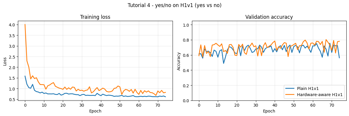
plot_histories(
{
"Plain H1v1": history_plain,
"Hardware-aware H1v1": history_hw,
},
title=f"Tutorial 4 - yes/no on H1v1 ({WORD_1} vs {WORD_2})",
)
=== Hardware-aware H1v1 training ===


/tmp/ipykernel_29633/4173640007.py:22: UserWarning: Frontend on chip uses 16 filters. Using a different amount of neurons 13 is allowed but not respecting the chip constraints.
  self.frontend = H1v1Frontend(


epoch 01 | loss=4.0004 | train=55.1% | val=59.0%
epoch 05 | loss=1.5991 | train=65.7% | val=62.0%
epoch 10 | loss=1.1880 | train=69.3% | val=75.5%
epoch 15 | loss=1.2341 | train=68.2% | val=66.0%
epoch 20 | loss=1.0003 | train=71.6% | val=59.7%
epoch 25 | loss=0.9689 | train=70.7% | val=63.0%
epoch 30 | loss=0.9098 | train=71.5% | val=70.9%
epoch 35 | loss=1.0847 | train=70.3% | val=72.0%
epoch 40 | loss=0.9050 | train=73.5% | val=76.4%
epoch 45 | loss=0.8431 | train=72.5% | val=73.3%
epoch 50 | loss=1.1213 | train=69.7% | val=72.2%
epoch 55 | loss=0.9371 | train=72.6% | val=72.3%
epoch 60 | loss=0.8181 | train=74.5% | val=75.6%
epoch 65 | loss=0.8342 | train=76.1% | val=73.8%
epoch 70 | loss=0.6803 | train=76.2% | val=73.1%
epoch 75 | loss=0.8218 | train=75.0% | val=78.0%
Best validation accuracy: 80.3%
7. Mismatch-aware H1v1 training
Every analog transistor and memory cell on chip is fabricated slightly differently. On H1v1 this shows up as random offsets on synaptic weights (empirical stddev ≈ 0.02) and per-neuron variation in leak currents. A model trained on a perfect-chip assumption behaves differently on every real chip instance.
Training with mismatch enabled exposes the network to a different simulated chip variation every batch — prepare_net resamples the noise each time — so the network learns to be robust to it.
H1v1Synapse(stddev=0.02)— Gaussian weight noise σ=0.02 per batch on the dense synapses (frontend mismatch disabled for stability).H1v1Layer(ileak_mismatch=True)— per-neuron leak variability sampled from empirical H1v1 distributions.
See nwavesdk/docs/100a/h1/chip-constraints.md for empirical mismatch parameters.
class H1v1YesNoNetMismatch(nn.Module):
    """H1v1YesNoNet with mismatch simulation enabled on all layers."""

    def __init__(self, n_channels, hidden_size=64, num_classes=2):
        super().__init__()
        self.device_flag = device_flag
        slope = fast_sigmoid(slope=25.0)

        self.frontend = H1v1Frontend(
            nb_inputs=n_channels,
            device=self.device_flag,
            quantization_bit=5,
            stddev=0,
        )
        self.frontend_layer = H1v1Layer(
            n_neurons=n_channels,
            taus=10e-3,
            dt=8e-3,
            spike_grad=slope,
            device=self.device_flag,
            ileak_mismatch=False,
        )
        self.syn_hidden = H1v1Synapse(
            n_channels,
            hidden_size,
            device=self.device_flag,
            quantization_bit=5,
            stddev=0.02,
        )
        self.hidden = H1v1Layer(
            n_neurons=hidden_size,
            taus=64e-3,
            dt=8e-3,
            spike_grad=slope,
            device=self.device_flag,
            ileak_mismatch=True,
        )
        self.syn_out = H1v1Synapse(
            hidden_size,
            num_classes,
            device=self.device_flag,
            quantization_bit=5,
            stddev=0.02,
        )
        self.out = H1v1Layer(
            n_neurons=num_classes,
            taus=64e-3,
            dt=8e-3,
            spike_grad=slope,
            device=self.device_flag,
            ileak_mismatch=True,
        )

        self.frontend_stage = (self.frontend, self.frontend_layer)
        self.layer_pairs = [(self.syn_hidden, self.hidden), (self.syn_out, self.out)]

    def forward(self, x):
        prepare_net(self, collect_metrics=False)

        if self.device_flag == "gpu":
            cur0 = self.frontend(x)
            spk0, _ = self.frontend_layer(cur0)
            cur1 = self.syn_hidden(spk0)
            spk1, _ = self.hidden(cur1)
            cur2 = self.syn_out(spk1)
            spk2, _ = self.out(cur2)
            self.frontend_trace = spk0
            self.hidden_trace = spk1
            self.output_trace = spk2
            return spk2

        frontend_spk = []
        hidden_spk = []
        output_spk = []

        for t in range(x.shape[1]):
            cur0 = self.frontend(x[:, t, :])
            spk0, _ = self.frontend_layer(cur0)
            cur1 = self.syn_hidden(spk0)
            spk1, _ = self.hidden(cur1)
            cur2 = self.syn_out(spk1)
            spk2, _ = self.out(cur2)
            frontend_spk.append(spk0)
            hidden_spk.append(spk1)
            output_spk.append(spk2)

        self.frontend_trace = torch.stack(frontend_spk, dim=1)
        self.hidden_trace = torch.stack(hidden_spk, dim=1)
        self.output_trace = torch.stack(output_spk, dim=1)
        return self.output_trace
model_h1_mismatch = H1v1YesNoNetMismatch(N_CHANNELS, hidden_size=HIDDEN_SIZE).to(device)
history_mismatch, best_mismatch = train_model(
    model_h1_mismatch,
    train_loader,
    val_loader,
    name="Mismatch-aware H1v1 training",
    epochs=EPOCHS,
    lam_topology=0.05,
    lam_fr=10.0,
    target_fr=0.15,
    limit=0.9,
)

plot_histories(
    {
        "Plain H1v1": history_plain,
        "Hardware-aware H1v1": history_hw,
        "Mismatch-aware H1v1": history_mismatch,
    },
    title=f"Tutorial 4 - yes/no on H1v1 ({WORD_1} vs {WORD_2})",
)

print(f"\nBest validation accuracies:")
print(f"  Plain H1v1:           {best_plain:.1%}")
print(f"  Hardware-aware H1v1:  {best_hw:.1%}")
print(f"  Mismatch-aware H1v1:  {best_mismatch:.1%}")
=== Mismatch-aware H1v1 training ===


/tmp/ipykernel_29633/3189389693.py:9: UserWarning: Frontend on chip uses 16 filters. Using a different amount of neurons 13 is allowed but not respecting the chip constraints.
  self.frontend = H1v1Frontend(
2026-04-27 16:59:12,579 - root - INFO - Synapse mismatch at stddev = 0 has now been enabled
2026-04-27 16:59:12,582 - root - INFO - Synapse mismatch at stddev = 0.02 has now been enabled
2026-04-27 16:59:12,591 - root - INFO - Synapse mismatch at stddev = 0.02 has now been enabled


epoch 01 | loss=4.7260 | train=55.8% | val=66.6%
epoch 05 | loss=2.8163 | train=59.0% | val=56.8%
epoch 10 | loss=2.4186 | train=58.9% | val=48.6%
epoch 15 | loss=1.6954 | train=63.2% | val=58.5%
epoch 20 | loss=1.3115 | train=66.8% | val=58.5%
epoch 25 | loss=1.4463 | train=63.9% | val=65.9%
epoch 30 | loss=1.3712 | train=66.1% | val=69.5%
epoch 35 | loss=1.3657 | train=67.0% | val=67.9%
epoch 40 | loss=1.4187 | train=64.0% | val=56.1%
epoch 45 | loss=1.2381 | train=64.7% | val=61.1%
epoch 50 | loss=1.5781 | train=64.4% | val=69.8%
epoch 55 | loss=1.0348 | train=70.1% | val=69.4%
epoch 60 | loss=1.0936 | train=67.3% | val=61.4%
epoch 65 | loss=1.0636 | train=66.8% | val=63.9%
epoch 70 | loss=0.9875 | train=68.9% | val=65.8%
epoch 75 | loss=1.1077 | train=67.8% | val=74.2%
Best validation accuracy: 74.9%
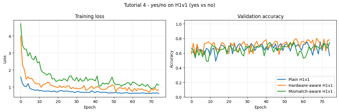
Best validation accuracies:
  Plain H1v1:           75.6%
  Hardware-aware H1v1:  80.3%
  Mismatch-aware H1v1:  74.9%
Three levels of hardware awareness
| Training variant | Quantization | Topology loss | Weight range loss | Mismatch simulation | Use when |
|---|---|---|---|---|---|
| Plain H1v1 | ✗ | ✗ | soft only | ✗ | Upper-bound benchmarking |
| Hardware-aware | ✓ (5-bit) | ✓ | soft + QAT clamp | ✗ | Deployment without mismatch characterization |
| Mismatch-aware | ✓ (5-bit) | ✓ | soft + QAT clamp | ✓ | Deployment on physical H1v1 hardware |
8. Summary
Three-step progression from simulation to hardware-ready:
| Plain H1v1 | Hardware-aware | Mismatch-aware | |
|---|---|---|---|
| Quantization | ✗ | 5-bit (32 levels) | 5-bit (32 levels) |
| Topology loss | ✗ | ✓ | ✓ |
| Weight magnitude loss | soft only | soft + QAT clamp | soft + QAT clamp |
| Mismatch simulation | ✗ | ✗ | ✓ |
| Chip-deployable | ✗ | ✓ | ✓ (most robust) |