NWAVE Tutorial 1: H1v1 Model hands-on overview

Tutorial by Giuseppe Gentile and Marco Rasetto

Overview

This tutorial introduces the two core neuron models in the NWAVE SDK:

LIFLayer: Flexible software LIF neuron, ideal for research and prototyping.
H1v1layer: Hardware-aware neuron that mirrors the constraints of the Neuronova H1v1 chip.

Understanding what can and cannot be changed in the H1v1 model is essential before training a network for deployment. Many parameters freely tunable in LIFLayer are fixed or absent in H1v1layer.

IMPORTANT

This was the first architecture developed at Neuronova and was initially used only internally. The evaluation kit will include the second version of H1. However, support for the first architecture is retained in later releases to allow teams who previously developed networks on it to continue using them as references and ensure backward compatibility. This architecture is planned to be deprecated and will not be supported in the future.

What You'll Learn

How LIFLayer dynamics depend on tau, threshold, and reset_mechanism
Which parameters are fixed, constrained, or absent in H1v1layer
Key physical differences: non-negative membrane, hardware leak currents, fixed network-wide threshold
How to interpret H1v1layer internal attributes

Experiment Setup

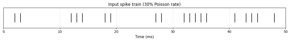
Input: single Poisson spike train (~30% rate, 100 ms, dt = 1 ms)
Neurons: 1 neuron per condition (isolated view of each effect)
No training: all cells are inference-only

1. Setup and Imports

import torch
import torch.nn as nn
import numpy as np
import matplotlib.pyplot as plt

from nwavesdk.layers import H1v1Synapse, H1v1Layer, LIFSynapse, LIFLayer, prepare_net

torch.manual_seed(42)
np.random.seed(42)

DT = 1e-3  # 1 ms timestep
T = 50  # 50 ms simulation

nwavesdk version: 1.0.0a0+cu


/opt/conda/envs/PyTorch/lib/python3.10/site-packages/tqdm/auto.py:21: TqdmWarning: IProgress not found. Please update jupyter and ipywidgets. See https://ipywidgets.readthedocs.io/en/stable/user_install.html
  from .autonotebook import tqdm as notebook_tqdm
2026-04-28 10:14:12,461 INFO util.py:154 -- Missing packages: ['ipywidgets']. Run `pip install -U ipywidgets`, then restart the notebook server for rich notebook output.
2026-04-28 10:14:12,732 INFO util.py:154 -- Missing packages: ['ipywidgets']. Run `pip install -U ipywidgets`, then restart the notebook server for rich notebook output.

2. Input Spike Train

A single Poisson-like spike train shared by all experiments. Each timestep fires independently at 30% probability.

torch.manual_seed(0)
input_spikes = (torch.rand(1, T, 1) < 0.30).float()  # [batch=1, T, features=1]
print(
    f"Spike train: {int(input_spikes.sum())} spikes over {T} ms  "
    f"(rate = {input_spikes.mean():.0%})"
)

t_ms = np.arange(T) * DT * 1000

fig, ax = plt.subplots(figsize=(12, 1.8))
ax.eventplot(
    np.where(input_spikes[0, :, 0].numpy())[0],
    lineoffsets=0,
    linelengths=0.8,
    color="black",
    linewidths=1.5,
)
ax.set_xlim(0, T)
ax.set_xlabel("Time (ms)", fontsize=11)
ax.set_title("Input spike train (30% Poisson rate)", fontsize=12)
ax.set_yticks([])
ax.grid(axis="x", alpha=0.3)
plt.tight_layout()
plt.show()

Spike train: 19 spikes over 50 ms  (rate = 38%)

png

3. LIF Model: Parameter Exploration

LIFLayer implements the discrete-time LIF neuron:

mem[t+1] = mem[t] x exp(-dt / tau)  +  I[t]

A spike fires when mem >= threshold, then the chosen reset_mechanism is applied.

All three parameters (tau, threshold, and reset_mechanism) are freely configurable.

# Helper: membrane traces + spike raster
def plot_traces(mems_dict, spks_dict, title, threshold_line=None):
    n = len(mems_dict)
    colors = plt.cm.viridis(np.linspace(0.1, 0.9, n))
    t = np.arange(len(next(iter(mems_dict.values())))) * DT * 1000

    fig, (ax1, ax2) = plt.subplots(
        2, 1, figsize=(12, 5), sharex=True, gridspec_kw={"height_ratios": [3, 1]}
    )
    for i, (lbl, mem) in enumerate(mems_dict.items()):
        ax1.plot(t, mem, label=lbl, color=colors[i], linewidth=1.8)
    if threshold_line is not None:
        ax1.axhline(
            threshold_line,
            color="crimson",
            linestyle="--",
            linewidth=1.2,
            alpha=0.7,
            label=f"threshold = {threshold_line}",
        )
    ax1.set_ylabel("Membrane potential")
    ax1.legend(loc="upper right", fontsize=9)
    ax1.grid(True, alpha=0.2)
    ax1.set_title(title)

    for i, (lbl, spks) in enumerate(spks_dict.items()):
        st = np.where(spks)[0]
        if len(st):
            ax2.eventplot(
                st, lineoffsets=i, linelengths=0.8, color=colors[i], linewidths=1.5
            )
    ax2.set_yticks(range(n))
    ax2.set_yticklabels(list(spks_dict.keys()), fontsize=8)
    ax2.set_xlabel("Time (ms)")
    ax2.set_ylabel("Spikes")
    ax2.grid(axis="x", alpha=0.2)
    plt.tight_layout()
    plt.show()

3a. Effect of Tau (τ) Membrane Time Constant

τ controls how quickly the membrane decays between spikes.

τ	Decay per ms `exp(-dt/τ)`	Behaviour
5 ms	0.819	Fast: responds only to recent spikes
50 ms	0.980	Slow: integrates over a long window

Larger τ → more temporal integration → smoother membrane → sparser, later spikes.

class LIFNet(nn.Module):
    def __init__(self, weight, tau, threshold=1, dt=DT, reset="subtraction"):
        super().__init__()
        _w = weight
        self.syn = LIFSynapse(1, 1, init=lambda w: nn.init.constant_(w, _w))
        self.lif = LIFLayer(
            1, taus=tau, thresholds=threshold, dt=dt, reset_mechanism=reset
        )

    def forward(self, x):
        self.eval()
        prepare_net(self)
        mems, spks = [], []
        for t in range(x.shape[1]):
            cur = self.syn(x[:, t, :])
            spk, mem = self.lif(cur)
            mems.append(mem[0, 0].item())
            spks.append(spk[0, 0].item())
        return np.array(mems), np.array(spks)

taus_to_test = {
    "tau=5ms": 5e-3,
    "tau=10ms": 10e-3,
    "tau=20ms": 20e-3,
    "tau=50ms": 50e-3,
}
W, THRESH = 0.5, 1.0

mems, spks = {}, {}
for lbl, tau in taus_to_test.items():
    lif = LIFNet(weight=W, tau=tau, dt=DT)
    mems[lbl], spks[lbl] = lif(input_spikes)

plot_traces(
    mems,
    spks,
    title="LIF: Effect of tau  (weight=0.5, threshold=1.0, reset=subtraction)",
    threshold_line=THRESH,
)

for lbl, s in spks.items():
    print(f"  {lbl}: spike rate = {s.mean():.1%}")

png

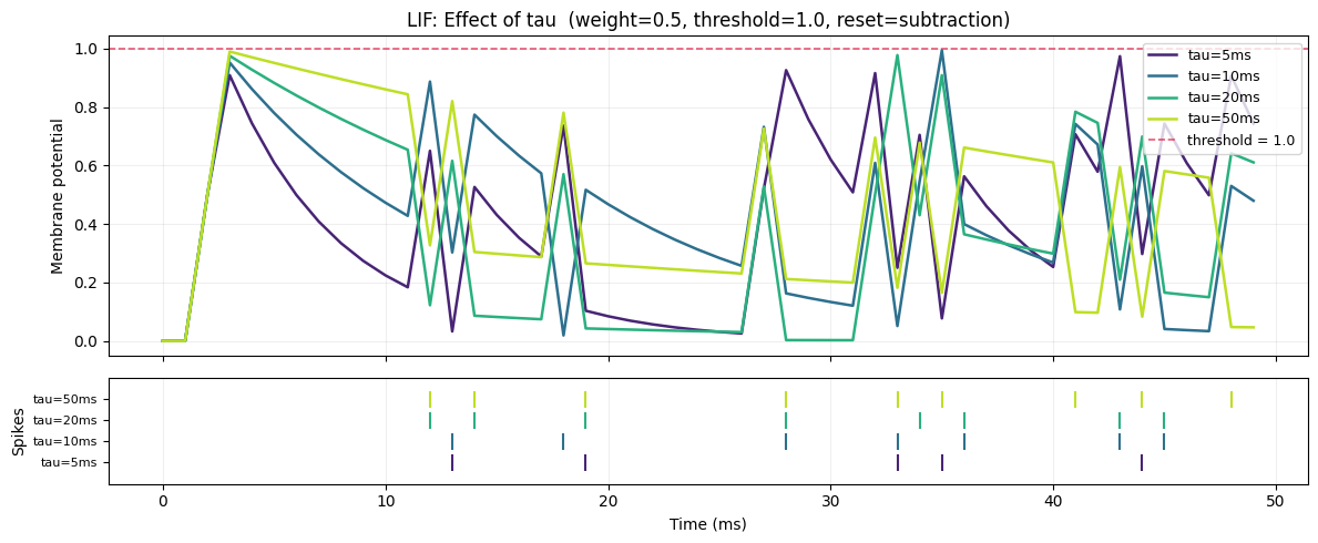
  tau=5ms: spike rate = 10.0%
  tau=10ms: spike rate = 14.0%
  tau=20ms: spike rate = 16.0%
  tau=50ms: spike rate = 18.0%

3b. Effect of Threshold (θ)

Threshold determines how much charge must accumulate before a spike fires.

Low θ → fires easily → high spike rate
High θ → selective → fires only on strong/persistent input

thresholds_to_test = {"th=0.3": 0.3, "th=0.6": 0.6, "th=1.0": 1.0, "th=2.0": 2.0}
W, TAU = 0.5, 20e-3

mems, spks = {}, {}
for lbl, thresh in thresholds_to_test.items():
    lif = LIFNet(weight=W, tau=TAU, threshold=thresh, dt=DT)
    mems[lbl], spks[lbl] = lif(input_spikes)

plot_traces(
    mems,
    spks,
    title="LIF: Effect of threshold  (weight=0.5, tau=20ms, reset=subtraction)",
)

for lbl, s in spks.items():
    print(f"  {lbl}: spike rate = {s.mean():.1%}")

png

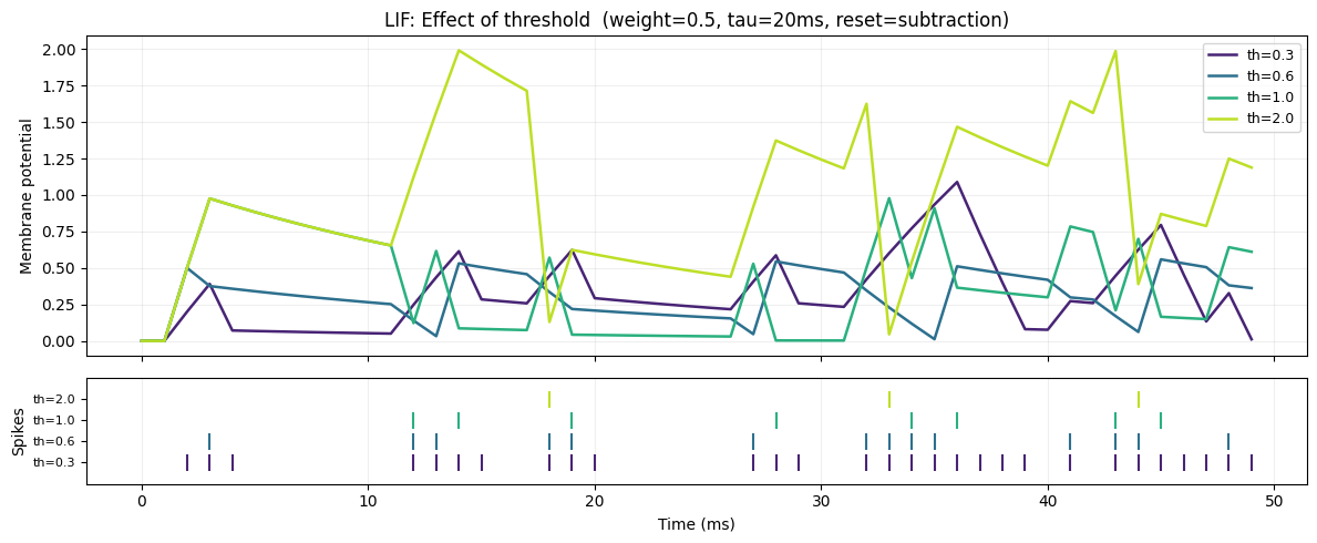
  th=0.3: spike rate = 58.0%
  th=0.6: spike rate = 28.0%
  th=1.0: spike rate = 16.0%
  th=2.0: spike rate = 6.0%

3c. Effect of Reset Mechanism

After a spike fires (mem >= threshold), LIFLayer applies one of three reset rules:

Mode	Rule	Effect
`"subtraction"`	`mem = mem - threshold`	Preserves excess charge above threshold
`"zero"`	`mem = 0`	Hard reset: discards all remaining charge
`"none"`	mem unchanged	No reset: membrane accumulates without bound

"subtraction" is the standard choice. "zero" is the closest reset to H1v1 behavior. "none" is useful for readout neurons where you want a continuous membrane signal.

W, TAU, THRESH = 0.5, 20e-3, 1.0

mems, spks = {}, {}
for reset in ["subtraction", "zero", "none"]:
    lif = LIFNet(weight=W, tau=TAU, dt=DT, reset=reset)

    mems[reset], spks[reset] = lif(input_spikes)

plot_traces(
    mems,
    spks,
    title="LIF: Effect of reset mechanism  (weight=0.5, tau=20ms, threshold=1.0)",
    threshold_line=THRESH,
)

for lbl, s in spks.items():
    print(f"  reset={lbl}: spike rate = {s.mean():.1%}")

png

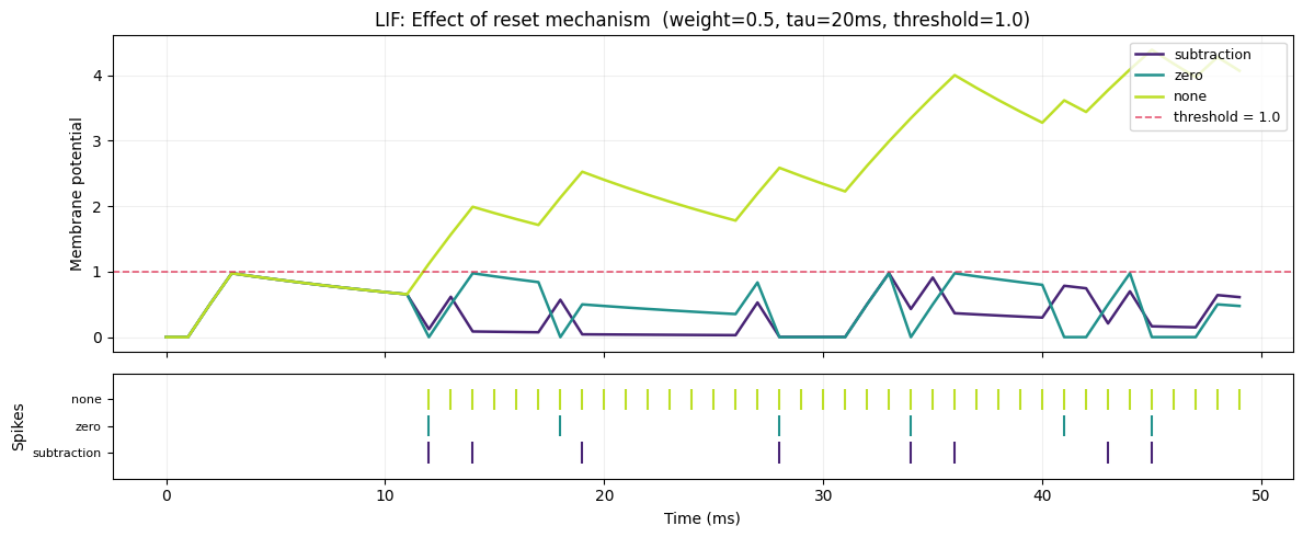
  reset=subtraction: spike rate = 16.0%
  reset=zero: spike rate = 12.0%
  reset=none: spike rate = 76.0%

3d. Learnable Taus and Thresholds

LIFLayer can make tau and threshold gradient-learnable:

learn_taus=True → stores decay factor _d_taus = exp(-dt/tau) as an nn.Parameter
learn_thresholds=True → stores thresholds as an nn.Parameter

This allows the network to discover optimal time constants during training. H1v1Layer has no equivalent (see Section 4a).

lif_learn = LIFLayer(
    5,
    taus=20e-3,
    thresholds=1.0,
    reset_mechanism="subtraction",
    dt=DT,
    learn_taus=True,
    learn_thresholds=True,
)

print("LIFLayer (learn_taus=True, learn_thresholds=True) - registered parameters:")
for name, p in lif_learn.named_parameters():
    print(f"  {name:<30} shape={tuple(p.shape)}  requires_grad={p.requires_grad}")

LIFLayer (learn_taus=True, learn_thresholds=True) - registered parameters:
  thresholds                     shape=(5,)  requires_grad=True
  _d_taus                        shape=(5,)  requires_grad=True

4. H1v1 Model: Hardware Constraints

H1v1Layer models the neuron circuits of the Neuronova H1v1 chip. It shares the same spike-generation rule but its membrane dynamics differ fundamentally from LIFLayer:

Constraint	LIFLayer	H1v1Layer
Decay type	Exponential: `mem *= exp(-dt/tau)`	Linear: `mem -= Vleak` (constant per step)
Tau	Any float, optionally learnable	Set at init -> `_Ileak`; not learnable
Threshold	Per-layer, optionally learnable	Fixed chip-wide, single value
Reset	`subtraction` / `zero` / `none`	Fixed (zero + non-negative clamp)
Membrane	Can go negative	Always >= 0
Variability	Not modelled	Optional `ileak_mismatch`

We explore each constraint below.

4a. Linear Decay and Hardware Leak Currents

The H1v1 model does not use exponential decay. Instead it uses a constant linear leak:

LIFLayer (exponential):  mem[t+1] = mem[t] * exp(-dt/tau)  +  I[t]
H1v1Layer  (linear):       mem[t+1] = max(0, mem[t] - Vleak  +  I[t])

where Vleak is a fixed voltage subtracted every timestep.

What "tau" means in each model:

	LIFLayer	H1v1Layer
Decay	Exponential	Linear
tau definition	Time for membrane to drop to `1/e ≈ 36.8%` of its value (standard RC time constant)	No single tau, leakage is set per step
Discharge time	Asymptotic (never fully reaches 0)	`threshold / Vleak` steps to reach 0 from `_vt` with no input
Weight dependence	tau is weight-independent	Apparent integration window grows with weight (larger charge -> higher peak -> longer drain)

Consequence: the tau argument in H1v1Layer does not map to the same concept as in LIFLayer. The table below shows, for each requested tau, the resulting Vleak per step and the full drain time: how long it takes for a neuron sitting exactly at the firing threshold (_vt) to reach zero membrane potential with no further input. This is threshold / Vleak, i.e. 100% discharge, not the 1/e drop used in LIF.

Learnability: H1v1Layer has no registered nn.Parameter. Contrast with LIFLayer (learn_taus=True) which stores the exponential decay factor _d_taus = exp(-dt/tau) as a trainable parameter.

4b. Threshold: Fixed Network-Wide

The Neuronova chip uses a single global firing threshold for all neurons. There is no per-layer or per-neuron threshold: it is a hardware property of the chip.

LIFLayer: each layer has its own threshold; optionally learnable
H1v1Layer: threshold is chip-level. Identical for every H1v1Layer in the network

# LIFLayer: per-layer, freely configurable
lif_a = LIFLayer(3, taus=20e-3, thresholds=0.5, reset_mechanism="subtraction", dt=DT)
lif_b = LIFLayer(3, taus=20e-3, thresholds=2.0, reset_mechanism="subtraction", dt=DT)
print("LIFLayer: per-layer configurable threshold:")
print(f"  Layer A threshold: {lif_a.thresholds[0].item():.2f}")
print(f"  Layer B threshold: {lif_b.thresholds[0].item():.2f}")
print()

# H1v1Layer: single chip-level threshold. Identical regardless of which layer you inspect
h1_a = H1v1Layer(3, taus=20e-3, dt=DT)
h1_b = H1v1Layer(3, taus=50e-3, dt=DT)  # different tau, but threshold is the same
print("H1v1Layer: chip-wide fixed threshold (same regardless of tau or layer):")
print(f"  Layer A (tau=20ms) _vt: {h1_a._vt:.4f}")
print(f"  Layer B (tau=50ms) _vt: {h1_b._vt:.4f}  <- same chip-level value")
print()
print("Note: there is no per-neuron or per-layer threshold override in H1v1Layer.")
print("      The threshold is a hardware property of the Neuronova H1v1 chip.")

LIFLayer: per-layer configurable threshold:
  Layer A threshold: 0.50
  Layer B threshold: 2.00

H1v1Layer: chip-wide fixed threshold (same regardless of tau or layer):
  Layer A (tau=20ms) _vt: 0.2040
  Layer B (tau=50ms) _vt: 0.2040  <- same chip-level value

Note: there is no per-neuron or per-layer threshold override in H1v1Layer.
      The threshold is a hardware property of the Neuronova H1v1 chip.

4c. Non-Negative Membrane Potential

The hardware clips membrane voltages at zero: analog circuits cannot hold negative charge.

LIFLayer allows negative membrane values (e.g. from inhibitory connections). H1v1Layer always clamps the membrane at 0.

To demonstrate, we apply an inhibitory input (negative synaptic weight) to both models.

INH_W = -0.8


class LIFInhib(nn.Module):
    def __init__(self):
        super().__init__()
        self.syn = LIFSynapse(1, 1, use_bias=False)
        self.lif = LIFLayer(
            1, taus=20e-3, thresholds=1.0, reset_mechanism="subtraction", dt=DT
        )
        with torch.no_grad():
            self.syn.weight.fill_(INH_W)

    def forward(self, x):
        prepare_net(self)
        mems = []
        for t in range(x.shape[1]):
            _, mem = self.lif(self.syn(x[:, t, :]))
            mems.append(mem[0, 0].item())
        return np.array(mems)


class H1Inhib(nn.Module):
    def __init__(self):
        super().__init__()
        _w = INH_W
        self.syn = H1v1Synapse(1, 1, init=lambda w: nn.init.constant_(w, _w))
        self.h1 = H1v1Layer(1, taus=20e-3, dt=DT)

    def forward(self, x):
        prepare_net(self)
        mems = []
        for t in range(x.shape[1]):
            _, mem = self.h1(self.syn(x[:, t, :]))
            mems.append(mem[0, 0].item())
        return np.array(mems)


with torch.no_grad():
    lif_mem = LIFInhib()(input_spikes)
    h1_mem = H1Inhib()(input_spikes)

fig, ax = plt.subplots(figsize=(12, 4))
ax.plot(
    t_ms, lif_mem, label="LIFLayer (can go below 0)", color="tab:blue", linewidth=1.8
)
ax.plot(
    t_ms,
    h1_mem,
    label="H1v1Layer  (clipped at 0)",
    color="tab:orange",
    linewidth=1.8,
    linestyle="--",
)
ax.axhline(0, color="black", linewidth=0.8, linestyle=":", alpha=0.6)
ax.fill_between(
    t_ms,
    np.minimum(lif_mem, 0),
    0,
    alpha=0.15,
    color="tab:blue",
    label="Negative region (LIF only)",
)
ax.set_xlabel("Time (ms)", fontsize=11)
ax.set_ylabel("Membrane potential", fontsize=11)
ax.set_title(
    "Non-negative membrane: inhibitory input (weight=-0.8), tau=20ms", fontsize=12
)
ax.legend(fontsize=10)
ax.grid(True, alpha=0.2)
plt.tight_layout()
plt.show()

print(f"LIF mem range: [{lif_mem.min():.4f},  {lif_mem.max():.4f}]")
print(f"H1v1  mem range: [{h1_mem.min():.4f},  {h1_mem.max():.4f}]  <- always >= 0")

png

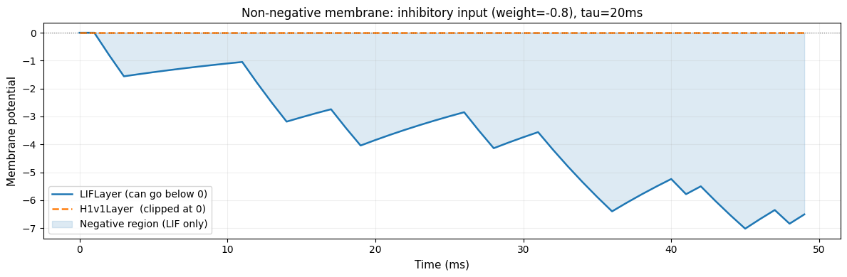
LIF mem range: [-7.0221,  0.0000]
H1v1  mem range: [0.0000,  0.0000]  <- always >= 0

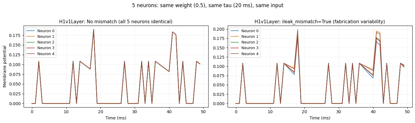
4d. Fabrication Variability (Mismatch)

Real neuromorphic chips exhibit device-to-device variability: even neurons with identical parameters behave slightly differently due to analog fabrication imperfections.

H1v1Layer models this with ileak_mismatch=True, adding calibrated noise to each neuron's effective leak current based on measured variability from the Neuronova H1v1 chip.

LIFLayer does not model mismatch, it is an idealised software simulation.

N, TAU_NOM, W = 5, 20e-3, 0.5


class H1Neurons(nn.Module):
    def __init__(self, mismatch):
        super().__init__()
        _w = W
        self.syn = H1v1Synapse(1, N, init=lambda w: nn.init.constant_(w, _w))
        self.h1 = H1v1Layer(N, taus=TAU_NOM, dt=DT, ileak_mismatch=mismatch)

    def forward(self, x):
        prepare_net(self)
        mems = []
        for t in range(x.shape[1]):
            _, mem = self.h1(self.syn(x[:, t, :]))
            mems.append(mem[0].detach().numpy().copy())
        return np.stack(mems)  # [T, N]


torch.manual_seed(7)
with torch.no_grad():
    mems_nom = H1Neurons(mismatch=False)(input_spikes)
    mems_mm = H1Neurons(mismatch=True)(input_spikes)

colors = plt.cm.tab10(np.linspace(0, 0.5, N))
fig, (ax1, ax2) = plt.subplots(1, 2, figsize=(14, 4))

for n in range(N):
    ax1.plot(t_ms, mems_nom[:, n], alpha=0.85, color=colors[n], label=f"Neuron {n}")
ax1.set_title("H1v1Layer: No mismatch (all 5 neurons identical)", fontsize=11)
ax1.set_xlabel("Time (ms)")
ax1.set_ylabel("Membrane potential")
ax1.legend(fontsize=9)
ax1.grid(True, alpha=0.2)

for n in range(N):
    ax2.plot(t_ms, mems_mm[:, n], alpha=0.85, color=colors[n], label=f"Neuron {n}")
ax2.set_title("H1v1Layer: ileak_mismatch=True (fabrication variability)", fontsize=11)
ax2.set_xlabel("Time (ms)")
ax2.legend(fontsize=9)
ax2.grid(True, alpha=0.2)

plt.suptitle(
    f"{N} neurons: same weight ({W}), same tau ({int(TAU_NOM*1000)} ms), same input",
    fontsize=12,
    y=1.02,
)
plt.tight_layout()
plt.show()

png

4e. Tau Quantisation

LIFLayer stores tau exactly as given.

H1v1Layer converts the requested tau into a hardware-native current leak Ileak, then transformed into a membrane voltage leak Vleak. The chip supports only a discrete set of tau values; requests are snapped to the nearest supported profile. Tau in this case is defined as a given drain time requested to complitely deplete a membrane voltage starting from the threshold.

Tau = _vt / Vleak × dt

tau_req = 10e-3

lif_snap = LIFLayer(
    n_neurons=1, taus=tau_req, thresholds=1.0, reset_mechanism="subtraction", dt=DT
)
h1_snap = H1v1Layer(n_neurons=1, taus=tau_req, dt=DT)

vleak = float(h1_snap.Vleak.mean().item())  # membrane potential drained per step
vt = float(h1_snap._vt.item())

print(f"Requested tau:      {tau_req * 1e3:.1f} ms")
print(f"LIF stored tau:     {float(lif_snap.taus.item()) * 1e3:.3f} ms  (exact)")
print(f"H1v1 Vleak/step:    {vleak:.6f}  (membrane drained per step)")
print(f"H1v1 drain time:    {vt / vleak * DT * 1e3:.1f} ms  (= _vt / Vleak × dt)")

Requested tau:      10.0 ms
LIF stored tau:     10.000 ms  (exact)
H1v1 Vleak/step:    0.013600  (membrane drained per step)
H1v1 drain time:    15.0 ms  (= _vt / Vleak × dt)

4f. Weight Constraints and Block-of-5 Sign Topology

Two additional constraints apply to H1v1 synaptic weights:

Magnitude: weights must lie within [-0.9, 0.9] (hardware voltage range). weight_magnitude_loss softly penalises out-of-range weights during training.
Sign topology: for each input neuron the output weights are partitioned into blocks of 5 — [0:5), [5:10), … — and all weights within a block must share the same sign. This mirrors the analog routing fabric of the chip.

SignAnnealing enforces the sign constraint by progressively hardening block-level sign agreement while keeping gradient flow through magnitudes. The same constraint and scheduler apply to H1v2 (see Tutorial 2 Section 7), with the weight range changed to [-1.66, 1.66].

from nwavesdk.optim import SignAnnealing


class ToyH1Net(nn.Module):
    def __init__(self, n_in, n_out):
        super().__init__()
        self.syn = H1v1Synapse(n_in, n_out)

    def forward(self, x):
        prepare_net(self)
        return torch.stack([self.syn(x[:, t, :]) for t in range(x.shape[1])], dim=1)


n_in, n_out = 12, 25
x_data = torch.randn(1, 128, n_in)
y_data = torch.randn(1, 128, n_out)

net = ToyH1Net(n_in, n_out)
W_initial = net.syn.weight.detach().clone()

epochs = 10
sign_annealer = SignAnnealing(net, total_epochs=epochs, alpha_start=0.5, alpha_end=12.0)
optimizer = torch.optim.Adam(net.parameters(), lr=1e-3)

for epoch in range(epochs):
    optimizer.zero_grad()
    nn.functional.mse_loss(net(x_data), y_data).backward()
    optimizer.step()
    sign_annealer.step(net, epoch)

W_final = net.syn.weight.detach().cpu()

fig, axes = plt.subplots(1, 2, figsize=(16, 4))
axes[0].imshow((W_initial.numpy() > 0), aspect="auto", cmap="gray_r")
axes[0].set_title("Before SignAnnealing")
axes[0].set_xlabel("Output neuron")
axes[0].set_ylabel("Input")
axes[1].imshow((W_final.numpy() > 0), aspect="auto", cmap="gray_r")
axes[1].set_title("After SignAnnealing (white = positive)")
axes[1].set_xlabel("Output neuron")
for c in range(0, 25, 5):
    axes[1].axvline(c - 0.5, color="red", linewidth=0.8)
plt.tight_layout()
plt.show()

print(
    f"Weight range after training: [{W_final.min():.3f}, {W_final.max():.3f}]  (limit: [-0.9, 0.9])"
)

png

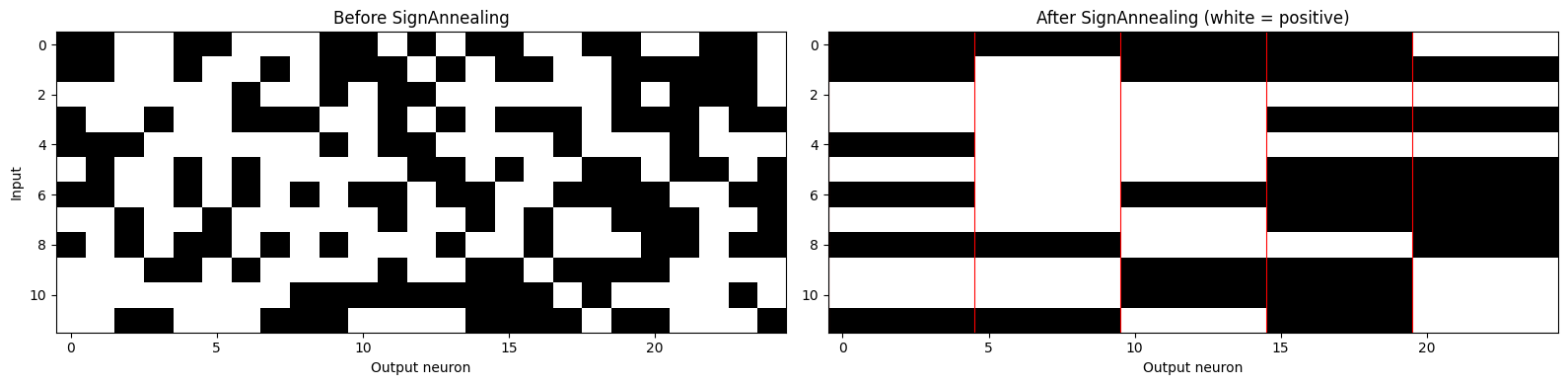
Weight range after training: [-0.366, 0.362]  (limit: [-0.9, 0.9])

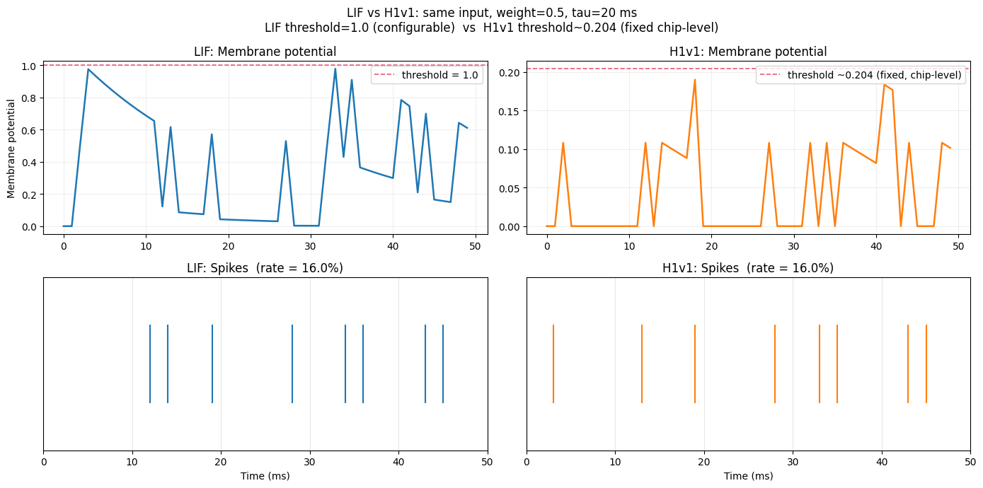
5. Side-by-Side: LIF vs H1v1

Both models receive the same input with the same weight and nominal tau. Differences arise purely from hardware constraints:

Threshold scale: H1v1 threshold is chip-level (~0.2 V); LIF uses 1.0 by default
Decay type: H1v1 uses linear decay (mem -= Vleak); LIF uses exponential (mem *= exp(-dt/tau))
Spike rate: follows from the threshold difference

class H1Net(nn.Module):
    def __init__(self, weight, tau, dt=DT):
        super().__init__()
        _w = weight
        self.syn = H1v1Synapse(1, 1, init=lambda w: nn.init.constant_(w, _w))
        self.h1 = H1v1Layer(1, taus=tau, dt=dt)

    def forward(self, x):
        self.eval()
        prepare_net(self)
        mems, spks = [], []
        for t in range(x.shape[1]):
            cur = self.syn(x[:, t, :])
            spk, mem = self.h1(cur)
            mems.append(mem[0, 0].item())
            spks.append(spk[0, 0].item())
        return np.array(mems), np.array(spks)

TAU, W = 20e-3, 0.5
h1 = H1Net(weight=W, tau=TAU, dt=DT)
lif = LIFNet(weight=W, tau=TAU, dt=DT)
lif_mem, lif_spks = lif(input_spikes)
h1_mem, h1_spks = h1(input_spikes)

h1_thresh = H1v1Layer(1, taus=TAU, dt=DT)._vt

fig, axes = plt.subplots(2, 2, figsize=(14, 7))

axes[0, 0].plot(t_ms, lif_mem, color="tab:blue", linewidth=1.8)
axes[0, 0].axhline(
    1.0,
    color="crimson",
    linestyle="--",
    linewidth=1.2,
    alpha=0.7,
    label="threshold = 1.0",
)
axes[0, 0].set_title("LIF: Membrane potential", fontsize=12)
axes[0, 0].set_ylabel("Membrane potential")
axes[0, 0].legend(fontsize=10)
axes[0, 0].grid(True, alpha=0.2)

axes[0, 1].plot(t_ms, h1_mem, color="tab:orange", linewidth=1.8)
axes[0, 1].axhline(
    h1_thresh,
    color="crimson",
    linestyle="--",
    linewidth=1.2,
    alpha=0.7,
    label=f"threshold ~{h1_thresh:.3f} (fixed, chip-level)",
)
axes[0, 1].set_title("H1v1: Membrane potential", fontsize=12)
axes[0, 1].legend(fontsize=10)
axes[0, 1].grid(True, alpha=0.2)

st_lif = np.where(lif_spks)[0]
axes[1, 0].eventplot(
    st_lif if len(st_lif) else [[-1]],
    lineoffsets=0,
    linelengths=0.8,
    color="tab:blue",
    linewidths=1.5,
)
axes[1, 0].set_title(f"LIF: Spikes  (rate = {lif_spks.mean():.1%})", fontsize=12)
axes[1, 0].set_xlabel("Time (ms)")
axes[1, 0].set_yticks([])
axes[1, 0].set_xlim(0, T)
axes[1, 0].grid(axis="x", alpha=0.3)

st_h1 = np.where(h1_spks)[0]
axes[1, 1].eventplot(
    st_h1 if len(st_h1) else [[-1]],
    lineoffsets=0,
    linelengths=0.8,
    color="tab:orange",
    linewidths=1.5,
)
axes[1, 1].set_title(f"H1v1: Spikes  (rate = {h1_spks.mean():.1%})", fontsize=12)
axes[1, 1].set_xlabel("Time (ms)")
axes[1, 1].set_yticks([])
axes[1, 1].set_xlim(0, T)
axes[1, 1].grid(axis="x", alpha=0.3)

plt.suptitle(
    f"LIF vs H1v1: same input, weight={W}, tau={int(TAU*1000)} ms\n"
    f"LIF threshold=1.0 (configurable)  vs  H1v1 threshold~{h1_thresh:.3f} (fixed chip-level)",
    fontsize=12,
)
plt.tight_layout()
plt.show()

png

6. Summary

Parameter / Feature	`LIFLayer`	`H1v1layer`
Tau (τ)	Any float; `learn_taus=True` stores `_d_taus` as `nn.Parameter`	Set at init -> `_Ileak`; not a gradient-learnable parameter
Threshold (θ)	Per-layer; `learn_thresholds=True` makes it learnable	Fixed chip-wide (`_vt`); same for all layers; not learnable
Reset mechanism	`subtraction` / `zero` / `none`	Fixed (zero + non-negative clamp)
Membrane polarity	Can go negative	Always >= 0 (hardware clamp)
Weight range	Unbounded	Bounded to `[-0.9, 0.9]`
Sign topology	No constraint	Groups of 5 weights must share sign
Device variability	Not modelled	`ileak_mismatch=True`, `stddev` available
Primary use case	Research, prototyping	Hardware deployment on Neuronova H1v1

Key Takeaways

Start with LIFLayer to explore ideas freely with full parameter control
Switch to H1v1layer when preparing for deployment
The threshold difference (LIF: 1.0 default, H1v1: ~0.2 chip-level) means you should scale weights/inputs accordingly when switching models
Enable ileak_mismatch=True during training for realistic performance estimates

Next Steps

Tutorial 2: Similar to this notebook, showcase of the H1v2 chip behavior and novelties with respect to H1v1.