NWAVE Tutorial 5: Audio Classification on H1v1 Hardware Model with Automatic Initialization
This tutorial keeps the same H1v1 architecture and hardware-aware training from Tutorial 4, but replaces the default initializations with automatic initializers built to ease the pain of initializing spiking neural networks.
It compares a default-initialized network against our automatic initializers.
1. Setup and Imports
import os
import shutil

import matplotlib.pyplot as plt
import numpy as np
import scipy.io.wavfile as wavfile
import torch
import torch.nn as nn
from torchaudio.datasets import SPEECHCOMMANDS

from nwavesdk import NWaveDataGen, NWaveDataloaderConfig
from nwavesdk.layers import H1v1Frontend, H1v1Synapse, H1v1Layer, prepare_net

# Our automatic initializers are in the init subsection of nwavesdk
from nwavesdk.init import fluct_init, frontend_firing_init

from nwavesdk.loss import (
    topology_loss,
    weight_magnitude_loss,
    firing_rate_target_mse_loss,
)
from nwavesdk.metrics import accuracy
from nwavesdk.surrogate import fast_sigmoid

from nwavesdk.init.hardware import init_weights


device = torch.device("cuda" if torch.cuda.is_available() else "cpu")
device_flag = "gpu" if device.type == "cuda" else "cpu"

torch.manual_seed(7)
np.random.seed(7)

print(f"Device: {device}")
nwavesdk version: 1.0.0a0+cu


/opt/conda/envs/PyTorch/lib/python3.10/site-packages/tqdm/auto.py:21: TqdmWarning: IProgress not found. Please update jupyter and ipywidgets. See https://ipywidgets.readthedocs.io/en/stable/user_install.html
  from .autonotebook import tqdm as notebook_tqdm
2026-04-28 10:35:41,153 INFO util.py:154 -- Missing packages: ['ipywidgets']. Run `pip install -U ipywidgets`, then restart the notebook server for rich notebook output.
2026-04-28 10:35:41,225 INFO util.py:154 -- Missing packages: ['ipywidgets']. Run `pip install -U ipywidgets`, then restart the notebook server for rich notebook output.


Device: cuda
2. Dataset and Preprocessing
Same dataset and preprocessing as Tutorial 4. If train_commands.pt and val_commands.pt already exist from a previous run, load them directly and skip the download cells below.
# ============================================
# CONFIGURATION: Choose your 2 words
# ============================================
# Available words in Speech Commands v0.02:
# yes, no, up, down, left, right, on, off, stop, go,
# zero, one, two, three, four, five, six, seven, eight, nine,
# bed, bird, cat, dog, happy, house, marvin, sheila, tree, wow

WORD_1 = "yes"  # Class 0
WORD_2 = "no"  # Class 1

# Audio parameters
SAMPLE_RATE = 16000  # Speech Commands native sample rate
RECORDING_DURATION_S = 1.0  # Each clip is 1 second

print(f"Training binary classifier: '{WORD_1}' (class 0) vs '{WORD_2}' (class 1)")
Training binary classifier: 'yes' (class 0) vs 'no' (class 1)
from torchaudio.datasets import SPEECHCOMMANDS

# Download Speech Commands dataset
os.makedirs("data", exist_ok=True)


class SubsetSpeechCommands(SPEECHCOMMANDS):
    """Speech Commands dataset filtered to specific words."""

    def __init__(self, root, subset, words, download=True):
        super().__init__(root, download=download, subset=subset)
        self.words = words
        # Filter to only include specified words
        self._walker = [
            item
            for item in self._walker
            if os.path.basename(os.path.dirname(item)) in words
        ]


# Load training and validation subsets
print(f"Downloading Speech Commands dataset (this may take a few minutes)...")
train_dataset = SubsetSpeechCommands("data", subset="training", words=[WORD_1, WORD_2])
val_dataset = SubsetSpeechCommands("data", subset="validation", words=[WORD_1, WORD_2])

print(f"\nDataset loaded:")
print(f"  Training samples: {len(train_dataset)}")
print(f"  Validation samples: {len(val_dataset)}")
Downloading Speech Commands dataset (this may take a few minutes)...

Dataset loaded:
  Training samples: 6358
  Validation samples: 803
import scipy.io.wavfile as wavfile

# Prepare data directory structure for NWaveDataGen
# NWaveDataGen expects: data_parent/class_name/*.wav

target_dir = "data_for_nwave_commands"
word1_dir = os.path.join(target_dir, WORD_1)
word2_dir = os.path.join(target_dir, WORD_2)

# Clean and create directories
if os.path.exists(target_dir):
    shutil.rmtree(target_dir)
os.makedirs(word1_dir, exist_ok=True)
os.makedirs(word2_dir, exist_ok=True)


def save_dataset_to_folders(dataset, word1_dir, word2_dir, word1, word2, prefix=""):
    """Save dataset samples to class folders as WAV files."""
    counts = {word1: 0, word2: 0}

    for i, (waveform, sample_rate, label, speaker_id, utterance_num) in enumerate(
        dataset
    ):
        # Determine output directory based on label
        if label == word1:
            out_dir = word1_dir
        elif label == word2:
            out_dir = word2_dir
        else:
            continue

        # Convert to numpy and ensure correct format
        audio = waveform.squeeze().numpy()

        # Pad or trim to exactly 1 second
        target_length = sample_rate  # 1 second
        if len(audio) < target_length:
            audio = np.pad(audio, (0, target_length - len(audio)))
        else:
            audio = audio[:target_length]

        # Convert to int16 for WAV file (scipy.io.wavfile format)
        audio_int16 = (audio * 32767).astype(np.int16)

        # Save file
        filename = f"{prefix}{label}_{speaker_id}_{utterance_num}_{i}.wav"
        filepath = os.path.join(out_dir, filename)
        wavfile.write(filepath, sample_rate, audio_int16)
        counts[label] += 1

    return counts


# Save training data
print("Preparing training data...")
train_counts = save_dataset_to_folders(
    train_dataset, word1_dir, word2_dir, WORD_1, WORD_2, prefix="train_"
)

# Save validation data
print("Preparing validation data...")
val_counts = save_dataset_to_folders(
    val_dataset, word1_dir, word2_dir, WORD_1, WORD_2, prefix="val_"
)

print(f"\nData prepared in '{target_dir}':")
print(f"  {WORD_1}/: {train_counts[WORD_1] + val_counts[WORD_1]} files")
print(f"  {WORD_2}/: {train_counts[WORD_2] + val_counts[WORD_2]} files")
Preparing training data...
Preparing validation data...

Data prepared in 'data_for_nwave_commands':
  yes/: 3625 files
  no/: 3536 files
from nwavesdk import NWaveDataGen, NWaveDataloaderConfig

data_config = NWaveDataloaderConfig(
    batch_size=16,
    val_split=0.15,
    test_split=0.0,
    random_state=123,
    num_workers=4,
    shuffle_train=True,
)

# Create data generator with hardware filterbank
dm = NWaveDataGen(
    data_parent=target_dir,
    sample_rate=SAMPLE_RATE,
    recording_duration_s=RECORDING_DURATION_S,
    sim_time_s=8e-3,  # 8ms time bins
    dataloader_config=data_config,
    task="classification",
    return_filename=True,
)

loaders = dm.dataloaders()
train_loader = loaders["train"]
val_loader = loaders["val"]

# Get number of filter channels from first batch
x, y, fn = next(iter(train_loader))
N_CHANNELS = x.shape[2]
print(f"\nInput shape: {x.shape} (batch, timesteps, channels)")
print(f"Number of filter channels: {N_CHANNELS}")
print(
    f"\nDataset split: {len(train_loader.dataset)} train, {len(val_loader.dataset)} validation"
)
2026-04-28 10:35:44,270 - root - WARNING - Using 13 valid freqs out of 16 for sr=16000Hz (Nyquist=8000.0Hz).
Classes (loading wavs): 100%|██████████| 2/2 [00:02<00:00,  1.11s/it]
Filtering no: 100%|██████████| 3536/3536 [00:00<00:00, 5181.63it/s]
Filtering yes: 100%|██████████| 3625/3625 [00:00<00:00, 4865.92it/s]


Input shape: torch.Size([16, 125, 13]) (batch, timesteps, channels)
Number of filter channels: 13

Dataset split: 6087 train, 1074 validation
# # (Optional) Save/Load dataloader
torch.save(train_loader, "train_commands.pt")
torch.save(val_loader, "val_commands.pt")

train_loader = torch.load("train_commands.pt", weights_only=False)
val_loader = torch.load("val_commands.pt", weights_only=False)
3. H1v1 model definition
Input → H1v1Frontend → H1v1Layer → H1v1Synapse → H1v1Layer → H1v1Synapse → H1v1Layer
Same architecture as Tutorial 4. prepare_net(model) must be called once per batch before the forward pass — it resets internal layer states and prepares hardware-specific buffers.
def dense_topology_penalty(model, lam):
    return topology_loss(model.syn_hidden, lam=lam) + topology_loss(
        model.syn_out, lam=lam
    )


class H1v1YesNoNet(nn.Module):
    """Frontend-first H1v1 classifier for yes/no keyword spotting."""

    def __init__(self, n_channels, hidden_size=64, num_classes=2, quantized=False):
        super().__init__()
        self.device_flag = device_flag
        slope = fast_sigmoid(slope=25.0)

        frontend_kwargs = {}
        dense_kwargs = {}
        if quantized:
            frontend_kwargs["quantization_bit"] = 5
            dense_kwargs["quantization_bit"] = 5

        self.frontend = H1v1Frontend(
            nb_inputs=n_channels,
            device=self.device_flag,
            **frontend_kwargs,
        )

        self.frontend_layer = H1v1Layer(
            n_neurons=n_channels,
            taus=10e-3,
            dt=8e-3,
            spike_grad=slope,
            device=self.device_flag,
        )
        self.syn_hidden = H1v1Synapse(
            n_channels,
            hidden_size,
            device=self.device_flag,
            **dense_kwargs,
        )
        self.hidden = H1v1Layer(
            n_neurons=hidden_size,
            taus=64e-3,
            dt=8e-3,
            spike_grad=slope,
            device=self.device_flag,
        )
        self.syn_out = H1v1Synapse(
            hidden_size,
            num_classes,
            device=self.device_flag,
            **dense_kwargs,
        )
        self.out = H1v1Layer(
            n_neurons=num_classes,
            taus=64e-3,
            dt=8e-3,
            spike_grad=slope,
            device=self.device_flag,
        )

        self.frontend_stage = (self.frontend, self.frontend_layer)
        self.layer_pairs = [(self.syn_hidden, self.hidden), (self.syn_out, self.out)]

    def forward(self, x):
        prepare_net(self, collect_metrics=False)

        if self.device_flag == "gpu":
            cur0 = self.frontend(x)
            spk0, _ = self.frontend_layer(cur0)
            cur1 = self.syn_hidden(spk0)
            spk1, _ = self.hidden(cur1)
            cur2 = self.syn_out(spk1)
            spk2, _ = self.out(cur2)
            self.frontend_trace = spk0
            self.hidden_trace = spk1
            self.output_trace = spk2
            return spk2

        frontend_spk = []
        hidden_spk = []
        output_spk = []

        for t in range(x.shape[1]):
            cur0 = self.frontend(x[:, t, :])
            spk0, _ = self.frontend_layer(cur0)
            cur1 = self.syn_hidden(spk0)
            spk1, _ = self.hidden(cur1)
            cur2 = self.syn_out(spk1)
            spk2, _ = self.out(cur2)
            frontend_spk.append(spk0)
            hidden_spk.append(spk1)
            output_spk.append(spk2)

        self.frontend_trace = torch.stack(frontend_spk, dim=1)
        self.hidden_trace = torch.stack(hidden_spk, dim=1)
        self.output_trace = torch.stack(output_spk, dim=1)
        return self.output_trace
4. Training utilities
def evaluate(model, loader):
    model.eval()
    correct = 0.0
    total = 0
    with torch.no_grad():
        for specs, labels, _ in loader:
            specs = specs.to(device)
            labels = labels.to(device)
            spike_traces = model(specs)
            correct += accuracy(spike_traces, labels)
            total += 1
    return correct / max(total, 1)


def train_model(
    model,
    train_loader,
    val_loader,
    *,
    name,
    epochs=20,
    lr_frontend=1e-5,
    lr_core=1e-3,
    lam_topology=0.0,
    lam_fr=0.0,
    target_fr=0.15,
    limit=0.9,
):
    criterion = nn.CrossEntropyLoss()
    optimizer = torch.optim.Adam(
        [
            {
                "params": list(model.frontend.parameters())
                + list(model.frontend_layer.parameters()),
                "lr": lr_frontend,
            },
            {
                "params": list(model.syn_hidden.parameters())
                + list(model.hidden.parameters())
                + list(model.syn_out.parameters())
                + list(model.out.parameters()),
                "lr": lr_core,
            },
        ]
    )

    history = {"train_loss": [], "train_acc": [], "val_acc": []}
    best_acc = 0.0
    best_state = None

    print(f"\n=== {name} ===")
    for epoch in range(1, epochs + 1):
        model.train()
        running_loss = 0.0
        running_correct = 0
        running_total = 0

        for specs, labels, _ in train_loader:
            specs = specs.to(device)
            labels = labels.to(device)

            optimizer.zero_grad()
            spike_traces = model(specs)
            logits = spike_traces.sum(dim=1)

            loss_main = criterion(logits, labels)
            loss_topo = (
                dense_topology_penalty(model, lam_topology)
                if lam_topology
                else torch.zeros((), device=logits.device)
            )
            loss_mag = weight_magnitude_loss(model, limit=limit)
            loss_fr = (
                firing_rate_target_mse_loss(
                    spikes_list=[spike_traces],
                    offsets=[target_fr],
                    multipliers=[lam_fr],
                )
                if lam_fr
                else torch.zeros((), device=logits.device)
            )

            loss = loss_main + loss_topo + loss_mag + loss_fr
            loss.backward()
            torch.nn.utils.clip_grad_norm_(model.parameters(), max_norm=0.5)
            optimizer.step()

            preds = logits.argmax(dim=1)
            running_correct += (preds == labels).sum().item()
            running_total += labels.size(0)
            running_loss += loss.item() * labels.size(0)

        train_acc = running_correct / max(running_total, 1)
        train_loss = running_loss / max(len(train_loader.dataset), 1)
        val_acc = evaluate(model, val_loader)

        history["train_loss"].append(train_loss)
        history["train_acc"].append(train_acc)
        history["val_acc"].append(val_acc)

        if val_acc >= best_acc:
            best_acc = val_acc
            best_state = {
                k: v.detach().cpu().clone() for k, v in model.state_dict().items()
            }

        if epoch == 1 or epoch % 5 == 0:
            print(
                f"epoch {epoch:02d} | loss={train_loss:.4f} | train={train_acc:.1%} | val={val_acc:.1%}"
            )

    if best_state is not None:
        model.load_state_dict(best_state)

    print(f"Best validation accuracy: {best_acc:.1%}")
    return history, best_acc


def plot_histories(histories, title):
    fig, axes = plt.subplots(1, 2, figsize=(12, 4))
    for label, history in histories.items():
        axes[0].plot(history["train_loss"], linewidth=2, label=label)
        axes[1].plot(history["val_acc"], linewidth=2, label=label)
    axes[0].set_title("Training loss")
    axes[0].set_xlabel("Epoch")
    axes[0].set_ylabel("Loss")
    axes[0].grid(True, alpha=0.3)
    axes[1].set_title("Validation accuracy")
    axes[1].set_xlabel("Epoch")
    axes[1].set_ylabel("Accuracy")
    axes[1].set_ylim(0.0, 1.05)
    axes[1].grid(True, alpha=0.3)
    axes[1].legend(loc="lower right")
    fig.suptitle(title)
    plt.tight_layout()
    plt.show()
5. Default initialisation vs automatic init
Default weight initialisation (Xavier or uniform) places neurons at an arbitrary operating point — some may start far from threshold and produce no gradient signal early in training.
frontend_firing_initbinary-searches frontend weights until the frontend layer fires at the target rate, preventing dead or always-firing frontend neurons.
frontend_firing_init finds the weights that will make frontend neurons fire close to the target firing rate, and then if quantization is present, re/quantizes the weights. For this reason final firing rate might depend on the precision required (if the target firing rate of 10% requires weights to be below the lowest bit, quantization might set them to 0, bringing firing rate to 0)
fluct_initsets dense synapse weights so the sub-threshold membrane variance is controlled and the mean sits close to threshold, maximising surrogate-gradient magnitude from the first batch.
fluct_init skips the H1v1Frontend → H1v1Layer stage because the frontend has diagonal (1-to-1) connectivity — weight variance cannot be meaningfully tuned with a single input per neuron. It initialises only the downstream dense H1v1Synapse → H1v1Layer pairs.
Both runs below use identical hardware-aware training from Tutorial 4; the only difference is the weight state before the first gradient step. Both initializers require the model and a dataloader to estimate the network's firing statistics on real data.
HIDDEN_SIZE = 64
EPOCHS = 50


def make_h1_model(seed):
    torch.manual_seed(seed)
    np.random.seed(seed)
    return H1v1YesNoNet(
        N_CHANNELS,
        hidden_size=HIDDEN_SIZE,
        quantized=True,
    ).to(device)


model_default = make_h1_model(seed=0)
model_fluct = make_h1_model(seed=0)

print("Running automatic initialization on the H1v1 network...")

frontend_firing_init(
    model_fluct,
    train_loader,
    target_fr=0.15,
    n_batches=8,  # Using 4 batches for a good ratio between stability and speed (we often need a small example of dataset statistics)
    verbose=True,
)

init_weights(
    model_fluct.frontend,
    init=(nn.init.normal_, {"mean": 0.1, "std": 0.01}),
)

fluct_init(
    model_fluct,
    train_loader,
    xi_target=3.0,
    alpha=1.0,
    n_batches=4,
    verbose=True,
)

history_default, best_default = train_model(
    model_default,
    train_loader,
    val_loader,
    name="Default init + hardware-aware H1v1 training",
    epochs=EPOCHS,
    lam_topology=0.05,
    lam_fr=10.0,
    target_fr=0.15,
    limit=0.9,
)

history_automatic, best_automatic = train_model(
    model_fluct,
    train_loader,
    val_loader,
    name="frontend_firing_init + fluct_init + hardware-aware H1v1 training",
    epochs=EPOCHS,
    lam_topology=0.05,
    lam_fr=10.0,
    target_fr=0.15,
    limit=0.9,
)

plot_histories(
    {
        "Default init": history_default,
        "Automatic init": history_automatic,
    },
    title=f"Tutorial 5 - H1v1 yes/no with automatic initialization ({WORD_1} vs {WORD_2})",
)

print(f"\nBest validation accuracy - default: {best_default:.1%}")
print(f"Best validation accuracy - automatic init: {best_automatic:.1%}")
Running automatic initialization on the H1v1 network...
[frontend_firing_init] target_fr=15.0%  n_batches=8  epsilon=2.0%  n_filters=13  [H1V1]


/tmp/ipykernel_8677/152967467.py:21: UserWarning: Frontend on chip uses 16 filters. Using a different amount of neurons 13 is allowed but not respecting the chip constraints.
  self.frontend = H1v1Frontend(


  neuron | w         fr(cont)  fr(quant)
  neuron  0 | w=0.0588  fr=0.150  →0.370  [OK  ]
  neuron  1 | w=0.0563  fr=0.150  →0.000  [OK  ]
  neuron  2 | w=0.0552  fr=0.150  →0.000  [OK  ]
  neuron  3 | w=0.0556  fr=0.150  →0.000  [OK  ]
  neuron  4 | w=0.0552  fr=0.150  →0.000  [OK  ]
  neuron  5 | w=0.0550  fr=0.150  →0.001  [OK  ]
  neuron  6 | w=0.0574  fr=0.150  →0.000  [OK  ]
  neuron  7 | w=0.0602  fr=0.150  →0.347  [OK  ]
  neuron  8 | w=0.0625  fr=0.150  →0.332  [OK  ]
  neuron  9 | w=0.0637  fr=0.150  →0.324  [OK  ]
  neuron 10 | w=0.0648  fr=0.150  →0.316  [OK  ]
  neuron 11 | w=0.0650  fr=0.150  →0.316  [OK  ]
  neuron 12 | w=0.0645  fr=0.150  →0.316  [OK  ]
[frontend_firing_init] done.
[fluct_init] ξ=3.0  α=1.0  dt=8.0ms  (stacked, adaptive µ)  [H1V1]
  Frontend stage skipped — nu_out=46.1Hz used as nu_in for layer 1
  Layer 1 | ν_in=46.1Hz  µ_W=0.0465  σ_FF=0.0440  µ_U=0.092
           → nu_2 = 19.0 Hz


/opt/conda/envs/PyTorch/lib/python3.10/site-packages/IPython/core/interactiveshell.py:3336: UserWarning: fluct_init layer 2: 2/2 neurons are dead after init. The fluctuation-driven regime (σ_FF > 0) requires µ_W ≤ 0.0314, but avoiding dead neurons needs µ_W > 0.0050. Consider a smaller ξ, lower α, or more input neurons (n_F=64).
  has_raised = await self.run_ast_nodes(code_ast.body, cell_name,


  Layer 2 | ν_in=19.0Hz  µ_W=0.0055  σ_FF=0.0728  µ_U=0.022
[fluct_init] done.

=== Default init + hardware-aware H1v1 training ===
epoch 01 | loss=4.3937 | train=55.0% | val=64.4%
epoch 05 | loss=1.3857 | train=64.4% | val=70.3%
epoch 10 | loss=1.0076 | train=68.6% | val=65.9%
epoch 15 | loss=0.7978 | train=74.1% | val=77.5%
epoch 20 | loss=0.8986 | train=71.3% | val=77.8%
epoch 25 | loss=0.8551 | train=72.3% | val=56.2%
epoch 30 | loss=0.8203 | train=74.0% | val=72.6%
epoch 35 | loss=0.7303 | train=75.3% | val=72.3%
epoch 40 | loss=0.7508 | train=76.0% | val=77.3%
epoch 45 | loss=0.7292 | train=75.4% | val=79.0%
epoch 50 | loss=0.8475 | train=74.1% | val=70.0%
Best validation accuracy: 79.3%

=== frontend_firing_init + fluct_init + hardware-aware H1v1 training ===
epoch 01 | loss=1.3090 | train=76.2% | val=85.2%
epoch 05 | loss=0.6598 | train=84.5% | val=89.0%
epoch 10 | loss=0.6346 | train=85.8% | val=88.6%
epoch 15 | loss=0.5715 | train=86.2% | val=89.8%
epoch 20 | loss=0.5833 | train=86.4% | val=91.3%
epoch 25 | loss=0.5308 | train=87.1% | val=90.3%
epoch 30 | loss=0.4516 | train=88.2% | val=90.5%
epoch 35 | loss=0.4610 | train=88.5% | val=85.1%
epoch 40 | loss=0.4864 | train=88.6% | val=90.0%
epoch 45 | loss=0.5054 | train=88.2% | val=89.6%
epoch 50 | loss=0.4354 | train=88.7% | val=90.3%
Best validation accuracy: 91.3%
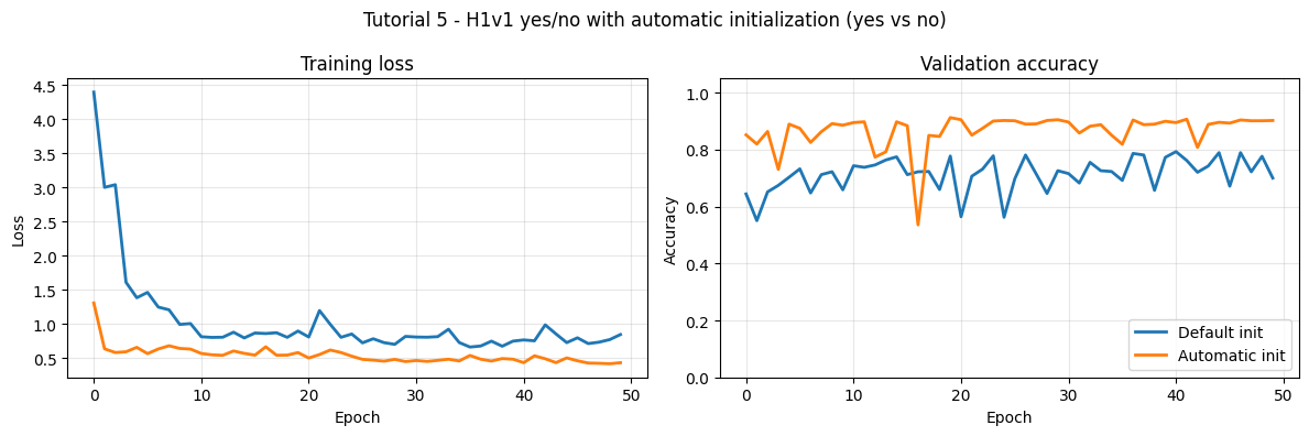
Best validation accuracy - default: 79.3%
Best validation accuracy - automatic init: 91.3%
6. Summary
frontend_firing_init + fluct_init start neurons close to threshold, reducing the risk of vanishing gradients in early training and lowering accuracy variance across random seeds. The initializers are data-driven: they require a few batches from the training loader to estimate firing statistics, but add negligible overhead before training begins.
For empirical parameter guidance see the initializations page on the official documentation.
Tutorial 6 applies the same initialization pipeline to the H1v2 chip, highlighting the parameter differences required by H1v2's lower synaptic gain.