NWAVE Tutorial 5: Recurrent Spiking Neural Networks

Tutorial by Giuseppe Gentile and Marco Rasetto

Overview

This tutorial introduces recurrent spiking neural networks (RSNNs) using the NWAVE SDK. We'll train a network to generate complex temporal patterns — a task that feedforward networks cannot solve.

What makes this task special?

We train the network to produce phase-shifted sinusoidal patterns across multiple output neurons. Each neuron must "remember" its phase and maintain rhythmic oscillations over time. Unlike regression (Tutorial 1) where outputs directly follow inputs, pattern generation requires internal memory:

Task Type	Memory Required	Network Type
Regression (Tutorial 1)	No — output follows input	Feedforward (`layer_topology="FF"`)
Pattern Generation	Yes — must maintain internal oscillation	Recurrent (`layer_topology="RC"`)

What You'll Learn

How to use layer_topology="RC" for recurrent connections
Why recurrent connections enable temporal pattern generation
Training RSNNs to produce multi-neuron oscillatory patterns
Visualizing learned recurrent dynamics

1. Setup and Imports

import torch
import torch.nn as nn
import numpy as np
import matplotlib.pyplot as plt
from tqdm import tqdm

from nwavesdk import LIFLayer, LIFSynapse, prepare_net
from nwavesdk.surrogate import fast_sigmoid

# Set random seeds for reproducibility
torch.manual_seed(42)
np.random.seed(42)

device = "cpu"

2. Target Pattern Generation

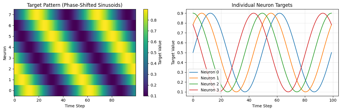
We generate sinusoidal target patterns with different phases for each output neuron. The network must learn to produce these oscillations autonomously — maintaining rhythm over time without external input driving the pattern.

Why can't feedforward networks do this?

A feedforward network's output is entirely determined by its current input. Given random noise input, a feedforward network produces random-looking output. Only with recurrent connections can the network maintain internal state and produce coherent temporal patterns.

def generate_temporal_targets(n_steps, n_neurons, pattern_type="sine"):
    """Generate phase-shifted sinusoidal targets for each neuron.

    Args:
        n_steps: Number of time steps
        n_neurons: Number of output neurons
        pattern_type: Type of pattern ("sine" supported)

    Returns:
        targets: Tensor of shape [n_steps, n_neurons] with values in [0.1, 0.9]
    """
    t = torch.linspace(0, 4 * np.pi, n_steps)
    targets = torch.zeros(n_steps, n_neurons)

    if pattern_type == "sine":
        for i in range(n_neurons):
            # Each neuron gets a different phase offset
            phase = (2 * np.pi * i) / n_neurons
            targets[:, i] = 0.5 + 0.4 * torch.sin(t + phase)

    return targets

# Hyperparameters
batch_size = 32
n_steps = 100       # 100ms simulation
n_neurons = 8       # 8 output neurons with different phases
dt = 1e-3           # 1ms timestep
taus = 10e-3        # 10ms membrane time constant
threshold = 0.1     # Low threshold for frequent spiking
surrogate_slope = 1.0
learning_rate = 0.001
n_epochs = 2000     # Needs sufficient epochs to converge

# Generate target patterns
target_pattern = generate_temporal_targets(n_steps, n_neurons, "sine").to(device)

print(f"Target shape: {target_pattern.shape}")
print(f"Target range: [{target_pattern.min():.2f}, {target_pattern.max():.2f}]")

# Visualize target patterns
plt.figure(figsize=(12, 4))
plt.subplot(1, 2, 1)
plt.imshow(target_pattern.T.numpy(), aspect='auto', cmap='viridis', origin='lower')
plt.colorbar(label='Target Value')
plt.xlabel('Time Step')
plt.ylabel('Neuron')
plt.title('Target Pattern (Phase-Shifted Sinusoids)')

plt.subplot(1, 2, 2)
for i in range(min(4, n_neurons)):
    plt.plot(target_pattern[:, i].numpy(), label=f'Neuron {i}')
plt.xlabel('Time Step')
plt.ylabel('Target Value')
plt.title('Individual Neuron Targets')
plt.legend()
plt.grid(True, alpha=0.3)
plt.tight_layout()
plt.show()

Target shape: torch.Size([100, 8])
Target range: [0.10, 0.90]

png

3. Model Definition: Recurrent LIF Network

Our pattern generator uses a simple but powerful architecture:

Architecture:

Input synapse: Transforms random noise input (1 → n_neurons)
Recurrent LIF layer: LIF neurons with recurrent connections (layer_topology="RC")

Key difference from Tutorial 1:

Tutorial 1 used layer_topology="FF" (feedforward only)
Here we use layer_topology="RC" which adds learnable recurrent connections

The recurrent weight matrix allows neurons to influence each other's activity, enabling the network to generate and sustain complex temporal dynamics.

class LIFPatternGenerator(nn.Module):
    """Recurrent SNN for temporal pattern generation.

    Architecture:
    - Input synapse: 1 -> n_neurons (transforms noise to each neuron)
    - Recurrent LIF: n_neurons with self-connections (RC topology)

    The recurrent connections enable sustained oscillatory patterns.
    """

    def __init__(self, n_neurons, taus, threshold, surrogate_slope, dt=1e-3):
        super().__init__()

        self.n_neurons = n_neurons

        # Input synapse: transforms scalar input to n_neurons
        # Random initialization breaks symmetry between neurons
        self.synapse = LIFSynapse(
            nb_inputs=1,
            nb_outputs=n_neurons,
            init=lambda w: nn.init.normal_(w, mean=0.5, std=0.1),
        )

        # Recurrent LIF layer - the key component!
        # layer_topology="RC" enables learnable recurrent weights
        self.lif = LIFLayer(
            n_neurons=n_neurons,
            taus=taus,
            dt=dt,
            thresholds=threshold,
            reset_mechanism="subtraction",
            layer_topology="RC",  # <-- This enables recurrence!
            spike_grad=fast_sigmoid(slope=surrogate_slope),
            init=lambda w: nn.init.normal_(w, mean=0.0, std=0.05),
        )

    def forward(self, x):
        """Forward pass through the recurrent network.

        Args:
            x: Input tensor [B, T, 1] - random spike train

        Returns:
            spikes: Output spikes [B, T, N]
            membrane: Membrane potentials [B, T, N]
        """
        B, T, _ = x.shape

        # Reset network state before each forward pass
        prepare_net(self, collect_metrics=False)

        spk_list = []
        mem_list = []

        # Process each timestep sequentially
        # Recurrent connections feedback from previous timestep
        for t in range(T):
            syn = self.synapse(x[:, t, :])  # Input current
            spk, mem = self.lif(syn)         # LIF dynamics + recurrence

            spk_list.append(spk)
            mem_list.append(mem)

        spikes = torch.stack(spk_list, dim=1)   # [B, T, N]
        membrane = torch.stack(mem_list, dim=1)

        return spikes, membrane

# Create the recurrent pattern generator
model = LIFPatternGenerator(
    n_neurons=n_neurons,
    taus=taus,
    threshold=threshold,
    surrogate_slope=surrogate_slope,
    dt=dt,
).to(device)

print("=== Model Architecture ===")
print(f"Input synapse shape: {model.synapse.weight.shape} (1 → {n_neurons})")
print(f"Recurrent weights shape: {model.lif.recurrent_weights.shape} ({n_neurons} × {n_neurons})")
print(f"Total parameters: {sum(p.numel() for p in model.parameters())}")
print(f"\nKey setting: layer_topology='RC' enables recurrent connections")

=== Model Architecture ===
Input synapse shape: torch.Size([1, 8]) (1 → 8)
Recurrent weights shape: torch.Size([8, 8]) (8 × 8)
Total parameters: 72

Key setting: layer_topology='RC' enables recurrent connections

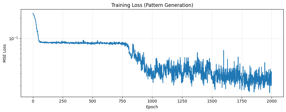
4. Training the Recurrent Network

We train the network to match batch-averaged spike patterns to the target sinusoids.

Training approach:

Input: Random spike train (40% probability per timestep)
Loss: MSE between batch-averaged output spikes and target pattern
Optimization: Adam optimizer on both input and recurrent weights

The key insight: even though input is random noise, the recurrent connections learn to produce structured temporal patterns.

# Training setup
optimizer = torch.optim.Adam(model.parameters(), lr=learning_rate)
model.train()
losses = []

for epoch in tqdm(range(n_epochs)):
    # Random input spikes (40% probability)
    x = (torch.rand(batch_size, n_steps, 1, device=device) > 0.6).float()

    # Forward pass
    y, h = model(x)

    # Loss: MSE between batch-averaged spikes and target
    y_mean = y.mean(dim=0)  # [T, N]
    loss = torch.nn.functional.mse_loss(y_mean, target_pattern)

    # Backward pass
    optimizer.zero_grad()
    loss.backward()
    optimizer.step()

    losses.append(loss.item())

    if (epoch + 1) % 200 == 0:
        print(f"Epoch {epoch+1:4d}/{n_epochs} | Loss: {loss.item():.6f}")

print(f"\nTraining complete! Final loss: {losses[-1]:.6f}")

 10%|█         | 205/2000 [00:10<00:38, 47.09it/s]

Epoch  200/2000 | Loss: 0.086802


 20%|██        | 405/2000 [00:14<00:27, 58.24it/s]

Epoch  400/2000 | Loss: 0.085010


 30%|███       | 604/2000 [00:18<00:17, 79.11it/s]

Epoch  600/2000 | Loss: 0.085540


 41%|████      | 814/2000 [00:21<00:13, 88.26it/s]

Epoch  800/2000 | Loss: 0.077148


 50%|█████     | 1005/2000 [00:26<00:21, 46.30it/s]

Epoch 1000/2000 | Loss: 0.026241


 60%|██████    | 1209/2000 [00:30<00:11, 71.79it/s]

Epoch 1200/2000 | Loss: 0.038944


 70%|███████   | 1410/2000 [00:34<00:10, 57.86it/s]

Epoch 1400/2000 | Loss: 0.041312


 81%|████████  | 1611/2000 [00:38<00:06, 62.54it/s]

Epoch 1600/2000 | Loss: 0.027532


 90%|█████████ | 1806/2000 [00:42<00:03, 59.22it/s]

Epoch 1800/2000 | Loss: 0.020725


100%|██████████| 2000/2000 [00:45<00:00, 43.57it/s]

Epoch 2000/2000 | Loss: 0.019949

Training complete! Final loss: 0.019949

# Plot training loss
plt.figure(figsize=(10, 4))
plt.plot(losses, linewidth=1.5)
plt.xlabel('Epoch')
plt.ylabel('MSE Loss')
plt.title('Training Loss (Pattern Generation)')
plt.yscale('log')
plt.grid(True, alpha=0.3)
plt.tight_layout()
plt.show()

png

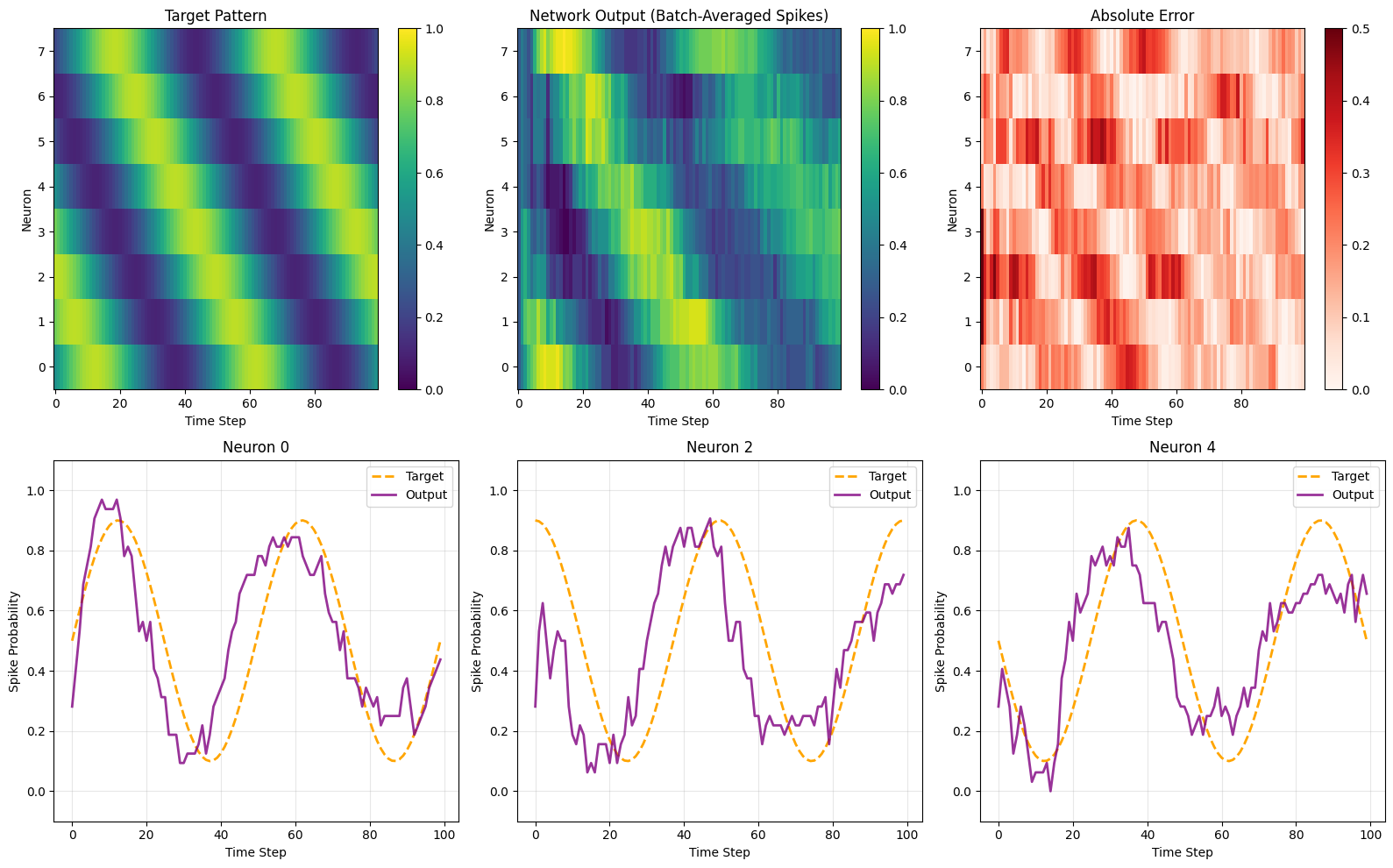
5. Evaluation

Let's evaluate how well the network learned to generate the target patterns.

# Evaluate the trained model
model.eval()
with torch.no_grad():
    # Generate new random input (different from training)
    x_test = (torch.rand(batch_size, n_steps, 1, device=device) > 0.6).float()
    y, h = model(x_test)
    output = y.mean(dim=0).cpu().numpy()  # Batch-averaged spikes

target_np = target_pattern.cpu().numpy()

# Compute metrics
mse = np.mean((output - target_np)**2)
mae = np.mean(np.abs(output - target_np))

print("=== Evaluation Metrics ===")
print(f"MSE: {mse:.6f}")
print(f"MAE: {mae:.6f}")

=== Evaluation Metrics ===
MSE: 0.034160
MAE: 0.153283

# Visualize results
fig = plt.figure(figsize=(16, 10))

# Target heatmap
plt.subplot(2, 3, 1)
plt.imshow(target_np.T, aspect='auto', cmap='viridis', origin='lower', vmin=0, vmax=1)
plt.xlabel('Time Step')
plt.ylabel('Neuron')
plt.title('Target Pattern')
plt.colorbar()

# Output heatmap
plt.subplot(2, 3, 2)
plt.imshow(output.T, aspect='auto', cmap='viridis', origin='lower', vmin=0, vmax=1)
plt.xlabel('Time Step')
plt.ylabel('Neuron')
plt.title('Network Output (Batch-Averaged Spikes)')
plt.colorbar()

# Error heatmap
plt.subplot(2, 3, 3)
error = np.abs(output - target_np)
plt.imshow(error.T, aspect='auto', cmap='Reds', origin='lower', vmin=0, vmax=0.5)
plt.xlabel('Time Step')
plt.ylabel('Neuron')
plt.title('Absolute Error')
plt.colorbar()

# Individual neuron traces
for i, neuron_idx in enumerate([0, 2, 4]):
    plt.subplot(2, 3, 4 + i)
    plt.plot(target_np[:, neuron_idx], '--', linewidth=2, label='Target', color='orange')
    plt.plot(output[:, neuron_idx], linewidth=2, label='Output', color='purple', alpha=0.8)
    plt.xlabel('Time Step')
    plt.ylabel('Spike Probability')
    plt.title(f'Neuron {neuron_idx}')
    plt.legend()
    plt.grid(True, alpha=0.3)
    plt.ylim([-0.1, 1.1])

plt.tight_layout()
plt.show()

png

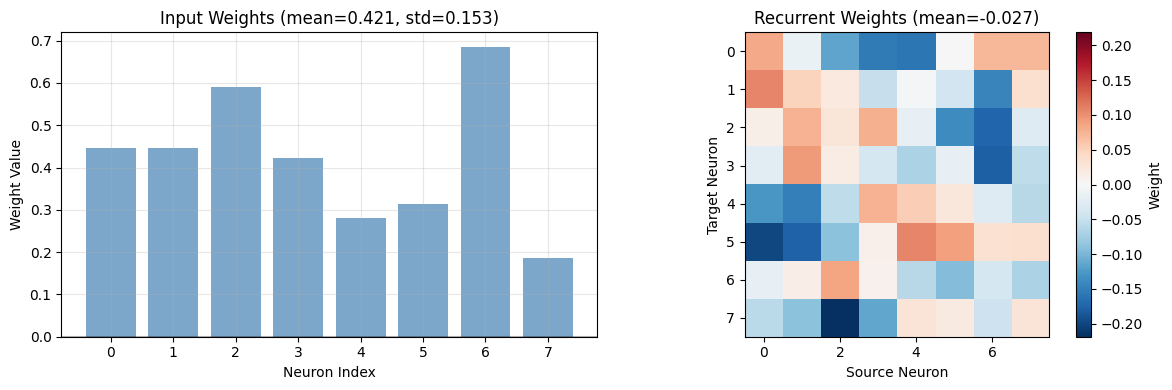
6. Analyzing Learned Weights

Let's examine the learned weights to understand how the network generates patterns:

Input weights (B): How each neuron responds to the random input
Recurrent weights (C): How neurons influence each other

# Extract learned weights
input_weights = model.synapse.weight.detach().cpu().numpy()
recurrent_weights = model.lif.recurrent_weights.detach().cpu().numpy()

fig, axes = plt.subplots(1, 2, figsize=(12, 4))

# Input weights (B): 1 → n_neurons
axes[0].bar(range(n_neurons), input_weights.flatten(), color='steelblue', alpha=0.7)
axes[0].set_xlabel('Neuron Index')
axes[0].set_ylabel('Weight Value')
axes[0].set_title(f'Input Weights (mean={input_weights.mean():.3f}, std={input_weights.std():.3f})')
axes[0].axhline(y=0, color='black', linestyle='-', alpha=0.3)
axes[0].grid(True, alpha=0.3)

# Recurrent weights (C): n_neurons × n_neurons
# Shows how each neuron (source, x-axis) affects each neuron (target, y-axis)
im = axes[1].imshow(recurrent_weights, cmap='RdBu_r', 
                    vmin=-np.abs(recurrent_weights).max(), 
                    vmax=np.abs(recurrent_weights).max())
axes[1].set_xlabel('Source Neuron')
axes[1].set_ylabel('Target Neuron')
axes[1].set_title(f'Recurrent Weights (mean={recurrent_weights.mean():.3f})')
plt.colorbar(im, ax=axes[1], label='Weight')

plt.tight_layout()
plt.show()

# Summary statistics
print(f"\n=== Weight Statistics ===")
print(f"Input weights:     mean={input_weights.mean():.4f}, std={input_weights.std():.4f}")
print(f"Recurrent weights: mean={recurrent_weights.mean():.4f}, std={recurrent_weights.std():.4f}")

png

=== Weight Statistics ===
Input weights:     mean=0.4214, std=0.1528
Recurrent weights: mean=-0.0275, std=0.0835

7. Summary

What We Learned

This tutorial demonstrated how to train recurrent spiking neural networks for temporal pattern generation:

Recurrent Connections (layer_topology="RC")
- Enable networks to maintain internal state and generate patterns autonomously
- Essential for tasks requiring memory (unlike feedforward networks)
Pattern Generation Task
- Network learns to produce phase-shifted sinusoidal patterns
- Each neuron learns a different oscillation phase
- Works despite random noise input
Key NWAVE Features
- layer_topology="RC" adds learnable recurrent weight matrix
- prepare_net() resets internal states between sequences
- Surrogate gradients enable backpropagation through spikes

Feedforward vs Recurrent: When to Use Each

Use Case	Topology	Example
Input-driven tasks	`"FF"`	Classification, regression
Pattern generation	`"RC"`	Oscillators, central pattern generators
Sequence memory	`"RC"`	Time series prediction, working memory

Next Steps

Experiment with different target patterns (square waves, complex rhythms)
Try deeper architectures with multiple recurrent layers
Explore longer time sequences