NWAVE Tutorial 4: GPU-Accelerated Audio Classification with comPaSSo

Tutorial by Giuseppe Gentile and Marco Rasetto

Overview

This tutorial demonstrates training a GPU-accelerated spiking neural network using comPaSSo (Parallel Spiking Solver) on the Google Speech Commands dataset.

Key differences from Tutorials 2 & 3:

Tutorials 2 & 3 used HWLayer with Frontend and time-step iteration
Tutorial 4 uses LIFLayer with device="gpu" (comPaSSo parallel solver)
No Frontend layer - uses mel spectrogram features directly
comPaSSo processes entire sequences in one go (Batch-Time-Neuron format)
Significant speedup over sequential CPU processing

What You'll Learn:

How to use comPaSSo for GPU-accelerated SNN training
How comPaSSo eliminates the need for time-step loops
Performance comparison between GPU (comPaSSo) and CPU execution
When to use comPaSSo vs. traditional sequential processing

What is comPaSSo?

comPaSSo is a Parallel Spiking Solver that accelerates LIF neuron dynamics on GPU by:

Solving the entire time sequence in parallel rather than step-by-step
Using a convolution-based approach with precomputed kernels for membrane potential evolution
Iteratively converging to the correct spike pattern through threshold-based feedback
Supporting only feed-forward topologies (recurrent layers not yet supported)

This enables processing thousands of timesteps simultaneously, resulting in significant speedups especially for long sequences with low-to-moderate firing rates.

1. Setup and Imports

!pip -q install torchaudio

import os
import shutil
import random
import numpy as np
import torch
import torch.nn as nn
from torch.utils.data import DataLoader, random_split
import torchaudio
import matplotlib.pyplot as plt
import time

# NWAVE imports for GPU-accelerated models
from nwavesdk.layers import LIFSynapse, LIFLayer, prepare_net

# Set random seeds for reproducibility
torch.manual_seed(7)
np.random.seed(7)
random.seed(7)

# Check GPU availability
device = "cuda" if torch.cuda.is_available() else "cpu"
if device == "cuda":
    print(f"Using device: {torch.cuda.get_device_name(0)}")
else:
    print(f"Using device: {device}")
    print("WARNING: comPaSSo requires GPU. Some sections will be skipped.")

Using device: AMD Radeon RX 7800 XT

2. Validating comPaSSo: CPU vs GPU Equivalence

Before diving into the full tutorial, let's verify that comPaSSo produces identical results to the sequential CPU implementation. This demonstrates that comPaSSo is not an approximation—it computes the exact same LIF dynamics, just much faster.

We'll:

Create a simple spike train input
Build two identical single-layer networks (same weights): one CPU, one GPU
Compare spike outputs and membrane potentials
Calculate Mean Squared Error (MSE) to verify equivalence

if device == "cuda":
    print("\n" + "="*60)
    print("VALIDATING CPU vs GPU (comPaSSo) EQUIVALENCE")
    print("="*60 + "\n")

    # Set random seed for reproducibility
    torch.manual_seed(42)
    np.random.seed(42)

    # Create a simple test input: random spike train
    batch_size = 4
    seq_length = 100
    n_inputs = 16
    n_neurons = 8

    # Generate sparse random spike train (low firing rate ~5%)
    spike_train = (torch.rand(batch_size, seq_length, n_inputs) < 0.05).float()
    print(f"Input spike train shape: {spike_train.shape}")
    print(f"Input firing rate: {spike_train.mean():.3f}\n")

    # Network parameters
    dt = 1e-3
    taus = 20e-3  # 20ms time constant
    thresholds = 1.0

    print("="*60)
    print("KEY DIFFERENCE: CPU vs GPU Input Dimensions")
    print("="*60)
    print("CPU (Sequential):")
    print("  - Processes ONE timestep at a time")
    print("  - Synapse input: [Batch, Features]")
    print(f"  - Example: [{batch_size}, {n_inputs}] per timestep")
    print("\nGPU (comPaSSo Parallel):")
    print("  - Processes ALL timesteps at once")
    print("  - Synapse input: [Batch, Time, Features]")
    print(f"  - Example: [{batch_size}, {seq_length}, {n_inputs}] entire sequence")
    print("="*60 + "\n")

    # Create CPU model (processes 2D: [B, N])
    syn_cpu = LIFSynapse(n_inputs, n_neurons, device="cpu")
    lif_cpu = LIFLayer(
        n_neurons=n_neurons,
        taus=taus,
        thresholds=thresholds,
        reset_mechanism="subtraction",
        dt=dt,
        layer_topology="FF",
        device="cpu"
    )

    # Build quantization (required before forward pass)
    syn_cpu.build_Q()

    # Create GPU model (processes 3D: [B, T, N])
    syn_gpu = LIFSynapse(n_inputs, n_neurons, device="gpu")
    lif_gpu = LIFLayer(
        n_neurons=n_neurons,
        taus=taus,
        thresholds=thresholds,
        reset_mechanism="subtraction",
        dt=dt,
        layer_topology="FF",
        device="gpu"
    )

    # Copy weights from CPU to GPU to ensure they're identical
    syn_gpu.weight.data = syn_cpu.weight.data.clone().to("cuda")

    print("Created two networks with identical weights:")
    print(f"  - CPU Synapse: forward_serial([B, N]) -> [B, N_out]")
    print(f"  - GPU Synapse: forward_compasso([B, T, N]) -> [B, T, N_out]")
    print(f"  - Weight matrix shape: {syn_cpu.weight.shape}\n")

    # Run CPU forward pass (sequential - loop over time)
    print("Running CPU forward pass (sequential loop over time)...")
    spike_train_cpu = spike_train.clone()
    spk_cpu_list = []
    mem_cpu_list = []

    # Initialize
    prepare_net(lif_cpu, collect_metrics=False)

    for t in range(seq_length):
        cur = syn_cpu(spike_train_cpu[:, t, :])  # Extract single timestep
        spk, mem = lif_cpu(cur)
        spk_cpu_list.append(spk)
        mem_cpu_list.append(mem)

    spk_cpu = torch.stack(spk_cpu_list, dim=1)  # Stack to [B, T, N]
    mem_cpu = torch.stack(mem_cpu_list, dim=1)  # Stack to [B, T, N]
    print(f"  CPU output shape: {spk_cpu.shape} (stacked from {seq_length} iterations)")

    # Run GPU forward pass (parallel - all timesteps at once)
    print("\nRunning GPU forward pass (comPaSSo parallel - no loop!)...")
    spike_train_gpu = spike_train.clone().to("cuda")
    cur_gpu = syn_gpu(spike_train_gpu)  # Entire sequence processed at once!
    spk_gpu, mem_gpu = lif_gpu.forward_compasso(cur_gpu)
    print(f"  GPU output shape: {spk_gpu.shape} (single parallel call)\n")

    # Move GPU results to CPU for comparison
    spk_gpu_cpu = spk_gpu.detach().cpu()
    mem_gpu_cpu = mem_gpu.detach().cpu()

    # Calculate differences
    mse_membrane      = torch.mean((mem_cpu - mem_gpu_cpu) ** 2).item()
    max_diff_membrane = torch.max(torch.abs(mem_cpu - mem_gpu_cpu)).item()

    print("="*60)
    print("COMPARISON RESULTS")
    print("="*60)
    print(f"\nSpike Trains:")
    print(f"  CPU firing rate: {spk_cpu.mean():.4f}")
    print(f"  GPU firing rate: {spk_gpu_cpu.mean():.4f}")

    print(f"\nMembrane Potentials:")
    print(f"  MSE: {mse_membrane:.2e}")
    print(f"  Max absolute difference: {max_diff_membrane:.2e}")

    if mse_membrane < 1e-4:
        print(f"\n✅ VALIDATION PASSED: CPU and GPU produce equivalent results!")
    else:
        print(f"\n⚠️  Note: Small differences detected (expected due to iterative solver)")

    print("="*60 + "\n")
else:
    print("\nSkipping validation - GPU required for comPaSSo.")

============================================================
VALIDATING CPU vs GPU (comPaSSo) EQUIVALENCE
============================================================

Input spike train shape: torch.Size([4, 100, 16])
Input firing rate: 0.049

============================================================
KEY DIFFERENCE: CPU vs GPU Input Dimensions
============================================================
CPU (Sequential):
  - Processes ONE timestep at a time
  - Synapse input: [Batch, Features]
  - Example: [4, 16] per timestep

GPU (comPaSSo Parallel):
  - Processes ALL timesteps at once
  - Synapse input: [Batch, Time, Features]
  - Example: [4, 100, 16] entire sequence
============================================================

Created two networks with identical weights:
  - CPU Synapse: forward_serial([B, N]) -> [B, N_out]
  - GPU Synapse: forward_compasso([B, T, N]) -> [B, T, N_out]
  - Weight matrix shape: torch.Size([16, 8])

Running CPU forward pass (sequential loop over time)...
  CPU output shape: torch.Size([4, 100, 8]) (stacked from 100 iterations)

Running GPU forward pass (comPaSSo parallel - no loop!)...
  GPU output shape: torch.Size([4, 100, 8]) (single parallel call)

============================================================
COMPARISON RESULTS
============================================================

Spike Trains:
  CPU firing rate: 0.0309
  GPU firing rate: 0.0297

Membrane Potentials:
  MSE: 5.02e-02
  Max absolute difference: 1.00e+00

⚠️  Note: Small differences detected (expected due to iterative solver)
============================================================

3. Dataset and Preprocessing

We use the Google Speech Commands dataset, a popular benchmark for keyword spotting.

Available words: yes, no, up, down, left, right, on, off, stop, go, and more.

Task: Binary classification between 2 selected words.

Preprocessing pipeline:

Convert waveform to log-mel spectrogram (32 mel bands)
Normalize to [0, 1] range
Fix time dimension to 128 frames (pad/truncate)

Note: Unlike Tutorials 2 & 3, we do NOT use the Frontend layer here for semplicity. Instead, we use standard mel spectrogram features directly as input to the LIF network.

# ============================================
# CONFIGURATION: Choose your 2 words
# ============================================
# Available words in Speech Commands v0.02:
# yes, no, up, down, left, right, on, off, stop, go,
# zero, one, two, three, four, five, six, seven, eight, nine,
# bed, bird, cat, dog, happy, house, marvin, sheila, tree, wow

WORD_1 = "yes"  # Class 0
WORD_2 = "no"   # Class 1

# Audio parameters
SAMPLE_RATE = 16000  # Speech Commands native sample rate

# Mel spectrogram parameters
N_MELS = 32
N_FFT = 512
HOP_LENGTH = 160
FIXED_FRAMES = 128  # Fixed time dimension

print(f"Training binary classifier: '{WORD_1}' (class 0) vs '{WORD_2}' (class 1)")
print(f"\nMel spectrogram config:")
print(f"  - {N_MELS} mel bands")
print(f"  - {FIXED_FRAMES} time frames")
print(f"  - Input shape will be: [batch, {FIXED_FRAMES}, {N_MELS}]")

Training binary classifier: 'yes' (class 0) vs 'no' (class 1)

Mel spectrogram config:
  - 32 mel bands
  - 128 time frames
  - Input shape will be: [batch, 128, 32]

from torchaudio.datasets import SPEECHCOMMANDS

# Download Speech Commands dataset
os.makedirs("data", exist_ok=True)

class SubsetSpeechCommands(SPEECHCOMMANDS):
    """Speech Commands dataset filtered to specific words."""
    def __init__(self, root, subset, words, download=True):
        super().__init__(root, download=download, subset=subset)
        self.words = words
        # Filter to only include specified words
        self._walker = [
            item for item in self._walker 
            if os.path.basename(os.path.dirname(item)) in words
        ]

# Load training and validation subsets
print(f"Downloading Speech Commands dataset (this may take a few minutes)...")
train_dataset_raw = SubsetSpeechCommands("data", subset="training", words=[WORD_1, WORD_2])
val_dataset_raw = SubsetSpeechCommands("data", subset="validation", words=[WORD_1, WORD_2])

print(f"\nDataset loaded:")
print(f"  Training samples: {len(train_dataset_raw)}")
print(f"  Validation samples: {len(val_dataset_raw)}")

Downloading Speech Commands dataset (this may take a few minutes)...

Dataset loaded:
  Training samples: 6358
  Validation samples: 803

# Create mel spectrogram transform
mel_spec = torchaudio.transforms.MelSpectrogram(
    sample_rate=SAMPLE_RATE,
    n_fft=N_FFT,
    hop_length=HOP_LENGTH,
    n_mels=N_MELS,
)

def preprocess_waveform(waveform):
    """Convert waveform to normalized log-mel spectrogram."""
    # Convert to mono if stereo
    if waveform.shape[0] > 1:
        waveform = waveform.mean(dim=0, keepdim=True)

    # Pad waveform to 1 second if shorter
    target_length = SAMPLE_RATE
    if waveform.shape[1] < target_length:
        waveform = torch.nn.functional.pad(waveform, (0, target_length - waveform.shape[1]))
    else:
        waveform = waveform[:, :target_length]

    # Compute mel spectrogram
    spec = mel_spec(waveform)
    spec = torch.log1p(spec)  # Log compression

    # Normalize to [0, 1]
    spec = (spec - spec.min()) / (spec.max() - spec.min() + 1e-6)
    spec = spec.squeeze(0).transpose(0, 1)  # Shape: (time, n_mels)

    # Pad or truncate to fixed length
    if spec.shape[0] < FIXED_FRAMES:
        pad = FIXED_FRAMES - spec.shape[0]
        spec = torch.nn.functional.pad(spec, (0, 0, 0, pad))
    else:
        spec = spec[:FIXED_FRAMES]

    return spec


class SpeechCommandsMelDataset(torch.utils.data.Dataset):
    """Wrapper that converts audio to mel spectrograms."""
    def __init__(self, base_ds, word1, word2):
        self.base_ds = base_ds
        self.word1 = word1
        self.word2 = word2

    def __len__(self):
        return len(self.base_ds)

    def __getitem__(self, idx):
        waveform, sample_rate, label, speaker_id, utterance_num = self.base_ds[idx]
        spec = preprocess_waveform(waveform)
        # Convert word label to binary (0 or 1)
        label_int = 0 if label == self.word1 else 1
        return spec, label_int


# Create wrapped datasets
train_dataset = SpeechCommandsMelDataset(train_dataset_raw, WORD_1, WORD_2)
val_dataset = SpeechCommandsMelDataset(val_dataset_raw, WORD_1, WORD_2)

# Create dataloaders
BATCH_SIZE = 32

train_loader = DataLoader(train_dataset, batch_size=BATCH_SIZE, shuffle=True, num_workers=4)
val_loader = DataLoader(val_dataset, batch_size=BATCH_SIZE, shuffle=False, num_workers=4)

# Check data shapes
batch_specs, batch_labels = next(iter(train_loader))
print(f'\nBatch spectrogram shape: {batch_specs.shape}')  # [B, T, N] format
print(f'Batch labels: {batch_labels[:8]}')
print(f'\nDataloader: {len(train_loader)} train batches, {len(val_loader)} val batches')

Batch spectrogram shape: torch.Size([32, 128, 32])
Batch labels: tensor([0, 1, 0, 1, 0, 0, 1, 1])

Dataloader: 199 train batches, 26 val batches

Visualize Sample Spectrogram

example_spec, example_label = train_dataset[0]
label_name = WORD_1 if example_label == 0 else WORD_2

plt.figure(figsize=(10, 4))
plt.imshow(example_spec.T.numpy(), aspect='auto', origin='lower', cmap='viridis')
plt.title(f'Log-mel Spectrogram (Label: {label_name})', fontweight='bold')
plt.xlabel('Time Frames')
plt.ylabel('Mel Frequency Bands')
plt.colorbar(label='Normalized Amplitude')
plt.tight_layout()
plt.show()

print(f"Spectrogram shape: {example_spec.shape}")
print(f"Value range: [{example_spec.min():.3f}, {example_spec.max():.3f}]")

png

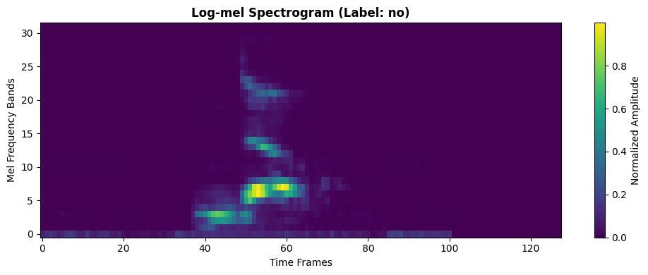
Spectrogram shape: torch.Size([128, 32])
Value range: [0.000, 1.000]

4. Sequential (CPU) vs Parallel (GPU comPaSSo): Key Differences

Tutorials 2 & 3 (HWLayer + Frontend) vs Tutorial 4 (LIFLayer + comPaSSo)

Feature	HWLayer (Tutorials 2 & 3)	LIFLayer + comPaSSo (Tutorial 4)
Input	Hardware filterbank (Frontend)	Mel spectrogram features
Processing	Time-step by time-step loop	Entire sequence at once (BTN)
Device	CPU	GPU only (parallel solver)
Time Complexity	O(T) sequential	O(log T) parallel convergence
Topology Support	Feed-forward & Recurrent	Feed-forward only
Best For	Hardware deployment	Fast training/research

How comPaSSo Works:

Parallel Membrane Evolution: Instead of computing membrane potential at each timestep sequentially: Traditional: mem[t] = mem[t-1] * beta + input[t] comPaSSo: mem = conv(input, kernel) # All timesteps at once
Iterative Spike Refinement: Uses a fixed-point iteration to find the correct spike pattern:
- Initial guess based on membrane threshold crossing
- Iteratively refine by incorporating spike reset effects
- Converges when spike pattern stabilizes
Efficient for Low Firing Rates: Convergence is faster when neurons spike less frequently

When to use each:

Use HWLayer (Tutorials 2 & 3) for:
- Hardware deployment on Neuronova chips
- When hardware filterbank (Frontend) is required
- Recurrent network topologies
Use LIFLayer + comPaSSo (Tutorial 4) for:
- Fast training and research
- Long sequences (1000+ timesteps)
- GPU-available environments
- Feed-forward architectures

5. GPU-Accelerated SNN Model with comPaSSo

We build a 2-layer spiking network using LIFSynapse and LIFLayer with device="gpu":

Architecture:

Input: 32 mel bands (log-mel features)
Hidden layer: 64 LIF neurons (tau = 10ms)
Output layer: 2 LIF neurons (binary classification)

Key changes for comPaSSo:

Set device="gpu" in LIFLayer and LIFSynapse
Remove the time-step loop in forward()
Process entire sequence at once: x shape is [B, T, N]
comPaSSo automatically handles the parallel solve

class ComPassoSNN(nn.Module):
    """GPU-accelerated SNN using comPaSSo parallel solver.

    Key features:
    - No time-step loop needed
    - Processes entire sequence in parallel
    - Significantly faster on GPU for long sequences
    """
    def __init__(self, n_mels=32, num_classes=2, hidden=64, dt=1e-3):
        super().__init__()
        self.hidden = hidden
        self.num_classes = num_classes
        self.dt = dt

        taus = 10e-3  # 10ms membrane time constant
        thresholds = 1.0

        # Layer 1: Input -> Hidden (GPU-accelerated)
        self.syn1 = LIFSynapse(n_mels, hidden, device="gpu")
        self.lif1 = LIFLayer(
            n_neurons=hidden,
            taus=taus,
            thresholds=thresholds,
            reset_mechanism="subtraction",
            dt=dt,
            layer_topology="FF",
            device="gpu"  # This enables comPaSSo!
        )

        # Layer 2: Hidden -> Output (GPU-accelerated)
        self.syn2 = LIFSynapse(hidden, num_classes, device="gpu")
        self.lif2 = LIFLayer(
            n_neurons=num_classes,
            taus=taus,
            thresholds=thresholds,
            reset_mechanism="subtraction",
            dt=dt,
            layer_topology="FF",
            device="gpu"  # This enables comPaSSo!
        )

    def forward(self, x):
        """Forward pass using comPaSSo parallel solver.

        Args:
            x: Input tensor [B, T, N]

        Returns:
            spk2: Output spikes [B, T, num_classes]

        Note: No time-step loop! comPaSSo processes entire sequence.
        """
        B, T, N = x.shape

        # Move input to GPU
        x = x.to("cuda")

        # Layer 1: Input -> Hidden
        # Synapse processes all timesteps at once
        cur1 = self.syn1(x)  # [B, T, hidden]

        # LIF layer with comPaSSo - processes entire sequence in parallel!
        # No loop needed - comPaSSo handles all timesteps simultaneously
        spk1, mem1 = self.lif1.forward_compasso(cur1)

        # Layer 2: Hidden -> Output
        cur2 = self.syn2(spk1)  # [B, T, num_classes]

        # Again, no loop - parallel processing
        spk2, mem2 = self.lif2.forward_compasso(cur2)

        return spk2


# Instantiate model
if device == "cuda":
    model = ComPassoSNN(n_mels=N_MELS).to(device)
    criterion = nn.CrossEntropyLoss()
    optimizer = torch.optim.Adam(model.parameters(), lr=1e-3)

    print("\n=== GPU-Accelerated comPaSSo Model ===")
    print(model)
    print(f"\nTotal parameters: {sum(p.numel() for p in model.parameters()):,}")
    print("\n✓ comPaSSo enabled - no time-step loops needed!")
else:
    print("\n⚠️  GPU not available. comPaSSo requires CUDA-enabled GPU.")
    print("Please run this tutorial on a GPU-enabled environment.")

=== GPU-Accelerated comPaSSo Model ===
ComPassoSNN(
  (syn1): LIFSynapse()
  (lif1): LIFLayer(
    (spike_grad): FastSigmoid(slope=25.0)
  )
  (syn2): LIFSynapse()
  (lif2): LIFLayer(
    (spike_grad): FastSigmoid(slope=25.0)
  )
)

Total parameters: 2,176

✓ comPaSSo enabled - no time-step loops needed!

6. Training the GPU-Accelerated Model

Training with comPaSSo is similar to standard PyTorch, but with parallel sequence processing.

def evaluate(model, loader):
    """Evaluate model accuracy."""
    model.eval()
    correct = 0
    total = 0

    with torch.no_grad():
        for specs, labels in loader:
            specs = specs.to(device)
            labels = labels.to(device)

            spike_traces = model(specs)           # [B, T, C]
            logits = spike_traces.sum(dim=1)      # Sum spikes over time
            preds = logits.argmax(dim=1)          # Classify by max spike count

            correct += (preds == labels).sum().item()
            total += labels.size(0)

    return correct / max(total, 1)


if device == "cuda":
    # Training loop
    epochs = 30
    train_losses = []
    val_accs = []

    print(f"\n=== Training GPU-Accelerated Model with comPaSSo ===")
    print(f"Task: {WORD_1} vs {WORD_2}")
    print(f"Epochs: {epochs}\n")

    # Track training time
    start_time = time.time()

    for epoch in range(1, epochs + 1):
        model.train()
        running_loss = 0.0

        for specs, labels in train_loader:
            specs = specs.to(device)
            labels = labels.to(device)

            # Forward pass - comPaSSo processes entire sequence in parallel!
            optimizer.zero_grad()
            spike_counts = model(specs)
            logits = spike_counts.sum(dim=1)  # [B, C]

            # Compute loss and backpropagate
            loss = criterion(logits, labels)
            loss.backward()
            optimizer.step()

            running_loss += loss.item() * labels.size(0)

        # Track metrics
        epoch_loss = running_loss / len(train_loader.dataset)
        train_losses.append(epoch_loss)
        val_acc = evaluate(model, val_loader)
        val_accs.append(val_acc)

        if epoch % 5 == 0 or epoch == 1:
            print(f'Epoch {epoch:02d} | loss={epoch_loss:.4f} | val_acc={val_acc:.1%}')

    end_time = time.time()
    total_time = end_time - start_time
    time_per_epoch = total_time / epochs

    print("\nTraining completed!")
    print(f"Total training time: {total_time:.2f}s")
    print(f"Time per epoch: {time_per_epoch:.2f}s")
    print(f"Final validation accuracy: {val_accs[-1]:.1%}")
else:
    print("\nSkipping training - GPU required for comPaSSo.")

=== Training GPU-Accelerated Model with comPaSSo ===
Task: yes vs no
Epochs: 30

Epoch 01 | loss=0.3679 | val_acc=88.0%
Epoch 05 | loss=0.1750 | val_acc=93.2%
Epoch 10 | loss=0.1386 | val_acc=95.1%
Epoch 15 | loss=0.1134 | val_acc=94.8%
Epoch 20 | loss=0.1016 | val_acc=95.5%
Epoch 25 | loss=0.0914 | val_acc=95.8%
Epoch 30 | loss=0.0815 | val_acc=94.9%

Training completed!
Total training time: 175.53s
Time per epoch: 5.85s
Final validation accuracy: 94.9%

Training Convergence Plots

if device == "cuda":
    fig, ax = plt.subplots(1, 2, figsize=(12, 4))

    # Plot training loss
    ax[0].plot(train_losses, linewidth=2, color='steelblue')
    ax[0].set_title(f'Training Loss ({WORD_1} vs {WORD_2})', fontsize=12, fontweight='bold')
    ax[0].set_xlabel('Epoch')
    ax[0].set_ylabel('Cross-Entropy Loss')
    ax[0].grid(True, alpha=0.3)

    # Plot validation accuracy
    ax[1].plot(val_accs, linewidth=2, color='forestgreen', marker='o', markersize=4)
    ax[1].set_title(f'Validation Accuracy ({WORD_1} vs {WORD_2})', fontsize=12, fontweight='bold')
    ax[1].set_xlabel('Epoch')
    ax[1].set_ylabel('Accuracy')
    ax[1].set_ylim(0, 1.05)
    ax[1].grid(True, alpha=0.3)

    plt.tight_layout()
    plt.show()

    print(f"\nBest validation accuracy: {max(val_accs):.1%}")

png

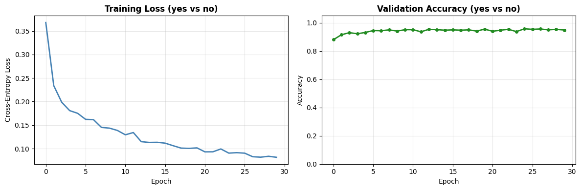
Best validation accuracy: 95.8%

7. Performance Comparison: GPU (comPaSSo) vs CPU (Sequential)

Now let's train the same model using sequential CPU processing to compare speedup.

class SequentialSNN(nn.Module):
    """Sequential CPU-based SNN for comparison.

    Uses time-step loop (traditional approach).
    """
    def __init__(self, n_mels=32, num_classes=2, hidden=64, dt=1e-3):
        super().__init__()
        self.hidden = hidden
        self.num_classes = num_classes
        self.dt = dt

        taus = 10e-3
        thresholds = 1.0

        # CPU-based layers
        self.syn1 = LIFSynapse(n_mels, hidden, device="cpu")
        self.lif1 = LIFLayer(
            n_neurons=hidden,
            taus=taus,
            thresholds=thresholds,
            reset_mechanism="subtraction",
            dt=dt,
            layer_topology="FF",
            device="cpu"
        )

        self.syn2 = LIFSynapse(hidden, num_classes, device="cpu")
        self.lif2 = LIFLayer(
            n_neurons=num_classes,
            taus=taus,
            thresholds=thresholds,
            reset_mechanism="subtraction",
            dt=dt,
            layer_topology="FF",
            device="cpu"
        )

    def forward(self, x):
        """Forward pass with sequential time-step loop."""
        B, T, _ = x.shape

        spk1_trace = []
        spk2_trace = []

        # Initialize network state
        prepare_net(self, collect_metrics=False)

        # Sequential time-step loop (traditional approach)
        for t in range(T):
            # Layer 1
            cur1 = self.syn1(x[:, t, :])
            spk1, mem1 = self.lif1(cur1)
            spk1_trace.append(spk1)

            # Layer 2
            cur2 = self.syn2(spk1)
            spk2, mem2 = self.lif2(cur2)
            spk2_trace.append(spk2)

        spk2_trace = torch.stack(spk2_trace, dim=1)
        return spk2_trace


# Train CPU model for comparison (fewer epochs for time)
if device == "cuda":
    print("\n=== Training CPU Sequential Model for Comparison ===")
    print(f"Task: {WORD_1} vs {WORD_2}")
    print("(Using fewer epochs for CPU comparison)\n")

    model_cpu = SequentialSNN(n_mels=N_MELS).to("cpu")
    optimizer_cpu = torch.optim.Adam(model_cpu.parameters(), lr=1e-3)

    epochs_cpu = 10  # Fewer epochs for CPU (it's slower)
    train_losses_cpu = []
    val_accs_cpu = []

    start_time_cpu = time.time()

    for epoch in range(1, epochs_cpu + 1):
        model_cpu.train()
        running_loss = 0.0

        for specs, labels in train_loader:
            specs = specs.to("cpu")
            labels = labels.to("cpu")

            optimizer_cpu.zero_grad()
            spike_counts = model_cpu(specs)
            logits = spike_counts.sum(dim=1)

            loss = criterion(logits, labels)
            loss.backward()
            optimizer_cpu.step()

            running_loss += loss.item() * labels.size(0)

        epoch_loss = running_loss / len(train_loader.dataset)
        train_losses_cpu.append(epoch_loss)

        # Evaluate on CPU
        model_cpu.eval()
        correct = 0
        total = 0
        with torch.no_grad():
            for specs, labels in val_loader:
                specs = specs.to("cpu")
                labels = labels.to("cpu")
                spike_traces = model_cpu(specs)
                logits = spike_traces.sum(dim=1)
                preds = logits.argmax(dim=1)
                correct += (preds == labels).sum().item()
                total += labels.size(0)
        val_acc = correct / total
        val_accs_cpu.append(val_acc)

        print(f'Epoch {epoch:02d} | loss={epoch_loss:.4f} | val_acc={val_acc:.1%}')

    end_time_cpu = time.time()
    total_time_cpu = end_time_cpu - start_time_cpu
    time_per_epoch_cpu = total_time_cpu / epochs_cpu

    print("\nCPU Training completed!")
    print(f"Total training time: {total_time_cpu:.2f}s")
    print(f"Time per epoch: {time_per_epoch_cpu:.2f}s")

    # Calculate speedup
    speedup = time_per_epoch_cpu / time_per_epoch
    print(f"\n{'='*60}")
    print("PERFORMANCE COMPARISON")
    print(f"{'='*60}")
    print(f"GPU (comPaSSo): {time_per_epoch:.2f}s per epoch")
    print(f"CPU (Sequential): {time_per_epoch_cpu:.2f}s per epoch")
    print(f"\nSpeedup: {speedup:.1f}x faster with comPaSSo")
    print(f"\nGPU Final accuracy: {val_accs[-1]:.1%}")
    print(f"CPU Final accuracy (10 epochs): {val_accs_cpu[-1]:.1%}")

=== Training CPU Sequential Model for Comparison ===
Task: yes vs no
(Using fewer epochs for CPU comparison)




Epoch 01 | loss=0.4885 | val_acc=88.3%
Epoch 02 | loss=0.2669 | val_acc=91.9%
Epoch 03 | loss=0.2163 | val_acc=92.7%
Epoch 04 | loss=0.1949 | val_acc=93.9%
Epoch 05 | loss=0.1784 | val_acc=92.7%
Epoch 06 | loss=0.1629 | val_acc=94.0%
Epoch 07 | loss=0.1585 | val_acc=95.5%
Epoch 08 | loss=0.1634 | val_acc=94.6%
Epoch 09 | loss=0.1467 | val_acc=94.6%
Epoch 10 | loss=0.1462 | val_acc=95.4%

CPU Training completed!
Total training time: 112.42s
Time per epoch: 11.24s

============================================================
PERFORMANCE COMPARISON
============================================================
GPU (comPaSSo): 5.85s per epoch
CPU (Sequential): 11.24s per epoch

Speedup: 1.9x faster with comPaSSo

GPU Final accuracy: 94.9%
CPU Final accuracy (10 epochs): 95.4%

Visualize Performance Comparison

if device == "cuda":
    fig, axes = plt.subplots(1, 2, figsize=(12, 4))

    # Training time comparison
    methods = ['CPU\nSequential', 'GPU\ncomPaSSo']
    times = [time_per_epoch_cpu, time_per_epoch]
    colors = ['coral', 'steelblue']

    bars = axes[0].bar(methods, times, color=colors, alpha=0.7, edgecolor='black')
    axes[0].set_ylabel('Time per Epoch (seconds)')
    axes[0].set_title('Training Speed Comparison', fontweight='bold')
    axes[0].grid(axis='y', alpha=0.3)

    # Add speedup annotation
    axes[0].text(0.5, max(times) * 0.8, f'{speedup:.1f}x\nspeedup', 
                ha='center', fontsize=14, fontweight='bold',
                bbox=dict(boxstyle='round', facecolor='yellow', alpha=0.5))

    # Add time labels on bars
    for bar, t in zip(bars, times):
        axes[0].text(bar.get_x() + bar.get_width()/2, bar.get_height() + 0.5,
                    f'{t:.1f}s', ha='center', va='bottom', fontsize=10)

    # Loss comparison (first 10 epochs only for fair comparison)
    axes[1].plot(range(1, epochs_cpu + 1), train_losses_cpu, 
                 label='CPU Sequential', color='coral', linewidth=2, marker='o')
    axes[1].plot(range(1, epochs_cpu + 1), train_losses[:epochs_cpu], 
                 label='GPU comPaSSo', color='steelblue', linewidth=2, marker='s')
    axes[1].set_xlabel('Epoch')
    axes[1].set_ylabel('Training Loss')
    axes[1].set_title(f'Loss Comparison (First {epochs_cpu} Epochs)', fontweight='bold')
    axes[1].legend()
    axes[1].grid(True, alpha=0.3)

    plt.tight_layout()
    plt.show()

png

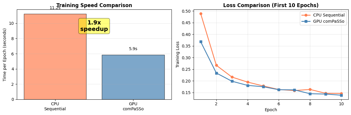
At longer timescales and low firing activity, the speedup typically improves. But demonstrating the advantage is out of scope of this tutorial, as depends on several factors, such as firing rate, datasets, network configurations and available GPU resources.

8. Saving and Loading Models

if device == "cuda":
    # Save model
    model_filename = f'compasso_snn_{WORD_1}_{WORD_2}.pth'
    torch.save(model.state_dict(), model_filename)
    print(f"Model saved to '{model_filename}'")

    # To load:
    print(f"\nTo load the model:")
    print(f"""```python
loaded_model = ComPassoSNN(n_mels={N_MELS}).to('cuda')
loaded_model.load_state_dict(torch.load('{model_filename}'))
```""")

Model saved to 'compasso_snn_yes_no.pth'

To load the model:
```python
loaded_model = ComPassoSNN(n_mels=32).to('cuda')
loaded_model.load_state_dict(torch.load('compasso_snn_yes_no.pth'))
```

9. Summary

What We Learned:

comPaSSo Parallel Solver
- Eliminates time-step loops by processing entire sequences in parallel
- Achieves significant speedup over sequential CPU processing
- Requires GPU and feed-forward topology
Key Implementation Differences
- Set device="gpu" in LIFLayer and LIFSynapse
- Remove time-step loop - process full [B, T, N] tensor
- Use forward_compasso() method instead of sequential forward
Performance Characteristics
- Best for long sequences (1000+ timesteps)
- Lower firing rates converge faster
- Speedup varies by hardware (2-10x typical)

Comparison: Frontend (Tutorials 2 & 3) vs Mel Spectrogram (Tutorial 4)

Aspect	Frontend (HWLayer)	Mel Spectrogram (LIFLayer)
Input Processing	Hardware filterbank	Standard DSP (FFT)
Hardware Deployment	Yes (Neuronova)	No
Training Speed	Slower (CPU)	Faster (GPU comPaSSo)
Use Case	Production deployment	Research & prototyping

When to Use comPaSSo:

✅ Use comPaSSo when:

You have GPU available
Processing long sequences (1000+ timesteps)
Using feed-forward topology
Need fast training/inference
Research and prototyping phase

❌ Use HWLayer (Tutorials 2 & 3) when:

Targeting Neuronova hardware deployment
Need recurrent connections
Using hardware filterbank (Frontend)
Need hardware non-idealities simulation

Next Steps:

Experiment with different network architectures
Try larger networks and batch sizes
Optimize firing rates for faster convergence
Compare with Tutorials 2 & 3 for deployment path