NWAVE Tutorial 1: Regression with Spiking Neural Networks

Tutorial by Giuseppe Gentile and Marco Rasetto

Overview

This tutorial will introduce you on using the NWAVE SDK for training Spiking Neural Networks (SNNs) on a simple task. We'll train a network to learn temporal functions (linear and square-root) and highlight key differences between NWAVE and the popular snnTorch library.

About NWAVE:

NWAVE is designed for training SNNs with hardware deployment in mind. It provides:

Hardware-ready models: Train SNNs that can be directly deployed on Neuronova's neuromorphic chips
Easy migration: Port existing networks from other frameworks with minimal code changes.
PyTorch compatibility: Standard [B, T, N] data format familiar to deep learning practitioners
Time series parallelization: Train LIF models via ComPaSSo, a GPU acceleration method to speed execution and training of SNNs

Reference: This tutorial follows a similar approach to the snnTorch regression tutorial to facilitate direct comparison.

What You'll Learn

How to create and train LIF(Leaky Integrate and Fire) SNNs using NWAVE
Key differences in data format between NWAVE and snnTorch
Training and evaluating SNNs for regression tasks
Performance monitoring and visualization

1. Setup and Imports

import torch
import torch.nn as nn
from torch.utils.data import DataLoader
import matplotlib.pyplot as plt
import numpy as np
import random
import tqdm

# NWAVE imports
from nwavesdk import LIFSynapse, LIFLayer, prepare_net

Set Random Seeds for Reproducibility

torch.manual_seed(42)
random.seed(42)
np.random.seed(42)

2. Dataset Generation

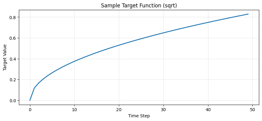
We create a simple regression dataset where the task is to learn temporal functions. The dataset generates linear trajectories from 0 to a random endpoint, and the target can be either:

Linear: Direct copy of the input
Square-root: Non-linear transformation of the input

This is identical to the snnTorch tutorial dataset for fair comparison.

class RegressionDataset(torch.utils.data.Dataset):
    """Simple regression dataset for temporal functions."""

    def __init__(self, timesteps, num_samples, mode):
        """Generate dataset with linear or square-root relationship.

        Args:
            timesteps: Number of time steps in each sequence
            num_samples: Number of samples to generate
            mode: 'linear' or 'sqrt' for the target function type
        """
        self.num_samples = num_samples
        feature_lst = []

        # Generate linear functions one by one
        for idx in range(num_samples):
            end = float(torch.rand(1))  # Random final point
            lin_vec = torch.linspace(start=0.0, end=end, steps=timesteps)
            feature = lin_vec.view(timesteps, 1)
            feature_lst.append(feature)

        self.features = torch.stack(feature_lst, dim=1)  # [T, B, N]

        # Generate labels based on mode
        if mode == "linear":
            self.labels = self.features * 1
        elif mode == "sqrt":
            slope = float(torch.rand(1))
            self.labels = torch.sqrt(self.features * slope)
        else:
            raise NotImplementedError("mode must be 'linear' or 'sqrt'")

    def __len__(self):
        return self.num_samples

    def __getitem__(self, idx):
        return self.features[:, idx, :], self.labels[:, idx, :]

Dataset Parameters and Visualization

sim_dt = 1e-3 # The dt in seconds for the simulation
num_steps = 50 # In the dt of the simulation, 50ms 
num_samples = 1024
mode = "sqrt"  # Options: 'linear' or 'sqrt'

# Generate dataset
dataset = RegressionDataset(timesteps=num_steps, num_samples=num_samples, mode=mode)

# Visualize a sample target function
sample = dataset.labels[:, 0, 0]
plt.figure(figsize=(10, 4))
plt.plot(sample, linewidth=2)
plt.title(f"Sample Target Function ({mode})")
plt.xlabel("Time Step")
plt.ylabel("Target Value")
plt.grid(True, alpha=0.3)
plt.show()

png

3. Key Difference: Data Format

NWAVE vs snnTorch Data Representation

This is one of the most important differences between the two frameworks:

Framework	Data Format	Description
snnTorch	`[T, B, N]`	Time-first format, aligns with SNN temporal processing
NWAVE	`[B, T, N]`	Batch-first format, consistent with standard PyTorch conventions

Where:

B: Batch size (number of samples)
T: Time steps (sequence length)
N: Features (dimensions per time step)

Why this matters:

snnTorch uses [T, B, N] because it processes spikes temporally, iterating over time steps first
NWAVE uses [B, T, N] to maintain consistency with standard deep learning frameworks (PyTorch RNNs, Transformers, etc.) and to facilitate easier integration with existing data pipelines

Hardware deployment advantage: The [B, T, N] format in NWAVE makes it easier to:

Port models from standard PyTorch implementations
Work with existing data processing pipelines
Prepare batches for efficient hardware deployment

In practice: When using data prepared for snnTorch with NWAVE, you need to permute dimensions from [T, B, N] to [B, T, N].

print(f"Original dataset shape (snnTorch format): {dataset.labels.shape}")
print(f"Format: [Time={dataset.labels.shape[0]}, Batch={dataset.labels.shape[1]}, Features={dataset.labels.shape[2]}]")

Original dataset shape (snnTorch format): torch.Size([50, 1024, 1])
Format: [Time=50, Batch=1024, Features=1]

Create DataLoader

The DataLoader will automatically handle the permutation when we iterate through batches.

batch_size = 32
dataloader = torch.utils.data.DataLoader(
    dataset=dataset, batch_size=batch_size, drop_last=True, shuffle=True
)

# Check the shape after DataLoader
sample_batch = next(iter(dataloader))
print(f"\nDataLoader output shape (NWAVE format): {sample_batch[0].shape}")
print(f"Format: [Batch={sample_batch[0].shape[0]}, Time={sample_batch[0].shape[1]}, Features={sample_batch[0].shape[2]}]")

DataLoader output shape (NWAVE format): torch.Size([32, 50, 1])
Format: [Batch=32, Time=50, Features=1]

4. Building the SNN Model

Network Architecture

We'll create a simple two-layer feedforward SNN using Leaky Integrate-and-Fire (LIF) neurons.

Model Parameters

input_size = 1   # Single-dimensional input
hidden_size = 256  # Hidden layer neurons
output_size = 1  # Single-dimensional output

# For ComPaSSo check ComPaSSo Tutorial
device = "cpu"   # NWAVE uses "gpu" if GPU available for GPU acceleration via ComPaSSo

5. Model Definition: NWAVE vs snnTorch

Key Architectural Differences

Aspect	snnTorch	NWAVE
Layer Structure	Separate `nn.Linear` + `snn.Leaky`	Combined `LIFSynapse` + `LIFLayer`
Time Loop	Manual loop over time steps	Manual loop over time steps
State Management	Returns (spikes, membrane)	Returns (spikes, membrane)
Bias Learning	Standard PyTorch	Explicit `bias_learn` parameter
Neuron Parameters	Abstract (beta decay)	Physical (tau, dt, threshold)
Reset Mechanism	Default subtract	Explicit `reset_mechanism` parameter
Data Format	`[T, B, N]` input	`[B, T, N]` input
Hardware Deployment	Simulation-focused	Hardware-ready models

Why we choose Physical Taus

NWAVE uses physical neuron parameters (time constants in seconds, simulation dt in seconds) instead of abstract parameters. This is critical for Hardware mapping as our analog solutions compute information in realtime on temporal scales in the order milliseconds, making hardware deployment more natural.

NWAVE Model Implementation

Understanding LIF Neuron Parameters

Before building the model, let's understand how the physical parameters in LIFLayer work:

The LIF Neuron Model

The Leaky Integrate-and-Fire neuron follows these dynamics:

# 1. Leaky Integration (membrane potential decay + input accumulation)
tau * dV/dt = -V + R*I(t)

# Discrete approximation:
V[t+1] = V[t] * exp(-dt/tau) + I[t]

Where:

V: Membrane potential (voltage)
tau (τ): Membrane time constant - how fast the neuron "forgets" past inputs
dt: Simulation time step
I(t): Input current at time t
R: Membrane resistance (absorbed into input current in practice)

# 2. Spike Generation
if V[t] >= threshold:
    spike = 1
else:
    spike = 0

# 3. Reset Mechanism
if spike == 1:
    V[t] = V[t] - threshold  # "subtraction" mode
    # OR
    V[t] = 0  # "zero" mode

Parameter Interpretation

Parameter	Typical Range	Biological Meaning	Effect on Network
tau	5-30 ms	Membrane time constant	Larger tau → slower response, more temporal integration
dt	0.1-1 ms	Simulation timestep	Smaller dt → more accurate but slower simulation
threshold	0.1-1.0	Spike threshold	Higher threshold → fewer spikes, harder to activate
reset_mechanism	"subtraction"	How membrane resets	"subtraction" preserves excess charge, "zero" discards it

Example Parameter Choices in This Tutorial

Hidden Layer (neu1):

taus = 16e-3         # 16ms - medium integration window
thresholds = 0.2     # Low threshold - easier to spike
dt = 1e-3            # 1ms timestep
reset = "subtraction"

Why 16ms tau? Good balance between responsiveness and temporal integration for the 50ms dataset
Why 0.2 threshold? Low enough to allow frequent spiking for learning
Why subtraction reset? Preserves information about "how much" threshold was exceeded

Output Layer (neu2):

taus = 1e-3          # 1ms - very fast (almost no memory)
thresholds = 10      # Very high - essentially won't spike!
dt = 1e-3
reset = "subtraction"

Why 1ms tau? Minimal temporal integration - acts like a "readout" layer
Why threshold=10? So high that it never spikes - we read the membrane potential, not spikes
Why this design? For regression, we want continuous outputs, so we use membrane voltage as the output signal

class NWaveRegressionNet(nn.Module):
    """NWAVE SNN for regression task.

    Architecture:
    - Layer 1: 1 -> 256 LIF neurons (hidden layer)
    - Layer 2: 256 -> 1 LIF neuron (output layer)
    """

    def __init__(self):
        super().__init__()

        # Layer 1: Input -> Hidden
        self.syn1 = LIFSynapse(input_size, hidden_size, use_bias=True, bias_learn=True)
        self.neu1 = LIFLayer(
            hidden_size,
            taus=16e-3,              # Time constant (16ms)
            thresholds=0.2,          # Spike threshold
            reset_mechanism="subtraction",  # Subtract threshold on spike
            dt=sim_dt                  # Time step (1ms)
        )

        # Layer 2: Hidden -> Output
        self.syn2 = LIFSynapse(hidden_size, output_size, use_bias=True, bias_learn=True)
        self.neu2 = LIFLayer(
            output_size,
            taus=1e-3,               # Shorter time constant for output
            thresholds=10,           # High threshold (membrane readout)
            reset_mechanism="subtraction",
            dt=sim_dt
        )

    def forward(self, x):
        """Forward pass through the network.

        Args:
            x: Input tensor of shape [B, T, N]

        Returns:
            spk_out: Output spikes [B, T, 1]
            mem_out: Output membrane potentials [B, T, 1]
            spk_hidden: Hidden layer spikes [B, T, hidden_size]
        """
        B, T, _ = x.shape

        mem_trace = []
        spk_trace = []
        spk_trace_hidden = []

        # Prepare network: Initialize hidden states (membrane potentials)
        # This MUST be called before the forward pass to reset internal states
        # Unlike snnTorch where you pass mem as input, NWAVE manages state internally
        prepare_net(self)

        # Time loop - process each time step
        for t in range(T):
            # Layer 1
            cur1 = self.syn1(x[:, t, :])  # Synaptic current
            spk1, mem1 = self.neu1(cur1)   # Neuron dynamics
            spk_trace_hidden.append(spk1)

            # Layer 2
            cur2 = self.syn2(spk1)
            spk2, mem2 = self.neu2(cur2)

            mem_trace.append(mem2)
            spk_trace.append(spk2)

        # Stack temporal outputs: [B, T, N]
        mem_trace = torch.stack(mem_trace, dim=1)
        spk_trace = torch.stack(spk_trace, dim=1)
        spk_trace_hidden = torch.stack(spk_trace_hidden, dim=1)

        return spk_trace, mem_trace, spk_trace_hidden


# Instantiate the model
model = NWaveRegressionNet().to(device)
print("\n=== Model Summary ===")
print(f"Total parameters: {sum(p.numel() for p in model.parameters()):,}")
print(f"Trainable parameters: {sum(p.numel() for p in model.parameters() if p.requires_grad):,}")

=== Model Summary ===
Total parameters: 769
Trainable parameters: 769

snnTorch Equivalent (for reference)

# This is how the same network would look in snnTorch:
import snntorch as snn

class SNNTorchRegressionNet(nn.Module):
    def __init__(self):
        super().__init__()

        # Layer 1
        self.fc1 = nn.Linear(input_size, hidden_size)
        self.lif1 = snn.Leaky(beta=0.9, init_hidden=True)

        # Layer 2
        self.fc2 = nn.Linear(hidden_size, output_size)
        self.lif2 = snn.Leaky(beta=0.9, init_hidden=True)

    def forward(self, x):
        # x shape: [T, B, N] for snnTorch

        # IMPORTANT: Manual state initialization in snnTorch
        mem1 = self.lif1.init_leaky()
        mem2 = self.lif2.init_leaky()

        spk_rec = []
        mem_rec = []

        for step in range(x.size(0)):  # Iterate over time
            cur1 = self.fc1(x[step])
            spk1, mem1 = self.lif1(cur1, mem1)  # Pass mem as input AND output!

            cur2 = self.fc2(spk1)
            spk2, mem2 = self.lif2(cur2, mem2)  # Manual state tracking

            spk_rec.append(spk2)
            mem_rec.append(mem2)

        return torch.stack(spk_rec), torch.stack(mem_rec)

Critical Differences:

State Management ⭐ Most Important Difference
- snnTorch: Manual state management - you must pass mem as both input and output python mem = lif.init_leaky() # Initialize spk, mem = lif(current, mem) # Pass mem explicitly
- NWAVE: Automatic internal state management - use prepare_net() once python prepare_net(model) # Initialize all layers spk, mem = lif(current) # No mem argument needed!
- Why it matters: NWAVE's approach is cleaner, less error-prone, and mirrors hardware behavior
Layer Architecture
- NWAVE: Separates synaptic connections (LIFSynapse) from neuron dynamics (LIFLayer)
- snnTorch: Combines both in standard nn.Linear followed by spiking neuron layers
- Why it matters: NWAVE's separation mirrors hardware architecture where synapses and neurons are distinct components
Neuron Parameters
- NWAVE: taus=16e-3 (16ms), dt=1e-3 (1ms), Physical values!
- snnTorch: beta=0.9 - Abstract decay parameter
- Conversion: beta = exp(-dt/tau), so tau ≈ -dt/log(beta) ≈ 9.5ms for beta=0.9, dt=1ms
- Why it matters: Physical parameters in NWAVE map directly to chip configurations
Data Format
- NWAVE: [B, T, N] - batch first (standard PyTorch)
- snnTorch: [T, B, N] - time first (SNN-specific)
- Why it matters: Easier to port existing PyTorch models to NWAVE
Function Calls Per Timestep
- NWAVE: prepare_net() once, then simple layer(input) calls
- snnTorch: Must track and pass mem variables for every neuron layer at every timestep
- Why it matters: NWAVE reduces boilerplate code and potential bugs

Migration from snnTorch to NWAVE - Quick Guide:

snnTorch Code	NWAVE Equivalent
`nn.Linear(in, out)` + `snn.Leaky(beta)`	`LIFSynapse(in, out)` + `LIFLayer(out, taus, thresholds, dt)`
`mem = lif.init_leaky()`	`prepare_net(model)` (once before forward)
`spk, mem = lif(cur, mem)`	`spk, mem = lif(cur)` (no mem argument!)
`x.shape = [T, B, N]`	`x.shape = [B, T, N]` (permute dimensions)
`beta = 0.9`	`tau = -dt/log(beta) ≈ 9.5ms` for dt=1ms

Understanding NWAVE SDK Functions

NWAVE provides specialized functions and layers that handle SNN simulation and state management differently from snnTorch. Here are the key components:

1. `LIFSynapse(nb_inputs, nb_outputs, use_bias, bias_learn)`

Purpose: Represents synaptic connections (weights) between neuron layers.

Parameters:

nb_inputs: Number of input neurons
nb_outputs: Number of output neurons
use_bias: Whether to include bias terms
bias_learn: Whether bias is trainable (separate from weight learning)

Key Features:

Implements weighted connections: output = input @ weights + bias
Supports quantization for hardware deployment (quantization_bits)
Xavier initialization for stable training
Can build quantized weights via build_Q() method

Hardware mapping: Synaptic weights map directly to crossbar arrays in neuromorphic chips.

2. `LIFLayer(n_neurons, taus, thresholds, reset_mechanism, dt, ...)`

Purpose: Implements Leaky Integrate-and-Fire neuron dynamics with internal state management.

Parameters:

n_neurons: Number of neurons in the layer
taus: Membrane time constant(s) in seconds (e.g., 16e-3 = 16ms)
thresholds: Spike threshold value(s)
reset_mechanism: How membrane resets after spike ("subtraction", "zero", or "none")
dt: Simulation time step in seconds (e.g., 1e-3 = 1ms)
spike_grad: Surrogate gradient function for backpropagation
layer_topology: "FF" (feedforward) or "RC" (recurrent)

Key Features:

Internal state management: Membrane potential is stored inside the layer (not passed as input!)
Reset mechanism options:
"subtraction": mem = mem - threshold (most common)
"zero": mem = 0 (hard reset)
"none": No reset (membrane keeps accumulating)

Mathematical model:

# Membrane dynamics (leaky integration):
mem_new = mem_old * exp(-dt/tau) + input_current

# Spike generation:
spike = 1 if mem_new >= threshold else 0

# Reset after spike:
mem_new = reset_function(mem_new, spike)

Hardware mapping:

tau and threshold directly configure analog neuron circuits
dt determines the discrete time step for digital event processing

3. `prepare_net(model)`

Purpose: Initializes/resets the network state before running a forward pass.

Why this is needed:

SNNs are stateful - neurons maintain membrane potentials across time steps
Must reset states between different input sequences (different batches)
Ensures clean state initialization for each forward pass

Key difference from snnTorch:

# snnTorch: Manual state management
mem1 = lif1.init_leaky()  # Initialize
for t in range(timesteps):
    spk, mem1 = lif1(cur, mem1)  # Pass mem as input/output

# NWAVE: Automatic state management  
prepare_net(model)  # Initialize once
for t in range(timesteps):
    spk, mem = lif_layer(cur)  # State managed internally!

Benefits:

Cleaner code - no need to track mem variables manually
Less error-prone - harder to forget state initialization
Better hardware alignment - mirrors how neuromorphic chips manage state

This internal state management is why you don't pass mem as an argument in NWAVE!

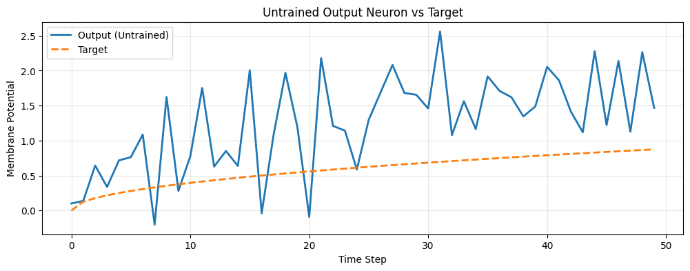
6. Untrained Network Behavior

Let's observe how the network behaves before training. The output should be random and not match the target.

Key Point: When to Call `prepare_net()`

The prepare_net() function is called inside the forward method in this tutorial because:

State Reset Between Sequences: Each batch is a different sequence, so we reset membrane potentials to zero
Metric Collection: We enable spike rate tracking for monitoring network activity
Clean Initialization: Ensures all neurons start from a known state

Important: In production or when processing multiple batches sequentially, you might want to:

Call prepare_net() once before the time loop (not inside)
Only reset between different input sequences, not between timesteps
Preserve state across timesteps within a sequence

Example patterns:

# Pattern 1: Reset per batch (as in this tutorial)
def forward(self, x):
    prepare_net(self, collect_metrics=True)  # Reset for each batch
    for t in range(T):
        spk, mem = self.neu(self.syn(x[:, t]))
    return spk, mem

# Pattern 2: Reset only at sequence start (more efficient)
prepare_net(model, collect_metrics=True)  # Call once before training
for batch in dataloader:
    output = model(batch)  # State persists across batches

# Pattern 3: Manual reset control
model.neu1.reset()  # Reset specific layer only

For this tutorial, we use Pattern 1 for clarity and to ensure clean state per forward pass.

# Get a batch of data
train_batch = iter(dataloader)
feature, label = next(train_batch)

# Run forward pass without gradients
with torch.no_grad():
    feature = feature.to(device)
    label = label.to(device)
    spk, mem, spk_h = model(feature)

# Visualize first sample
plt.figure(figsize=(12, 4))
plt.plot(mem[0, :, 0].cpu(), label="Output (Untrained)", linewidth=2)
plt.plot(label[0, :, 0].cpu(), "--", label="Target", linewidth=2)
plt.title("Untrained Output Neuron vs Target")
plt.xlabel("Time Step")
plt.ylabel("Membrane Potential")
plt.legend(loc="best")
plt.grid(True, alpha=0.3)
plt.show()

# Check initial spike rate
print(f"\nOutput layer spike rate: {spk.mean().item():.4f}")
print(f"Hidden layer spike rate: {spk_h.mean().item():.4f}")

png

Output layer spike rate: 0.0000
Hidden layer spike rate: 0.4659

7. Training the Network

Training Configuration

We'll train the network to minimize the Mean Squared Error (MSE) between the output membrane potential and the target function.

# Training hyperparameters
num_epochs = 150
learning_rate = 1e-2

# Optimizer and loss function
optimizer = torch.optim.AdamW(params=model.parameters(), lr=learning_rate)
loss_function = torch.nn.MSELoss()

loss_hist = []  # Track loss over time

# Training loop
model.train()
with tqdm.trange(num_epochs) as pbar:
    for epoch in pbar:
        epoch_loss = []

        for feature, label in dataloader:
            feature = feature.to(device)
            label = label.to(device)

            # Forward pass
            spk_out, mem_out, spk_hidden = model(feature)

            # Compute loss on membrane potential
            loss = loss_function(mem_out, label)

            # Backward pass
            optimizer.zero_grad()
            loss.backward()
            optimizer.step()

            # Record loss
            loss_hist.append(loss.item())
            epoch_loss.append(loss.item())

        # Update progress bar
        avg_loss = sum(epoch_loss) / len(epoch_loss)
        pbar.set_postfix(loss="%.3e" % avg_loss)

print("\nTraining completed!")

100%|██████████| 150/150 [00:37<00:00,  4.03it/s, loss=6.902e-04]


Training completed!

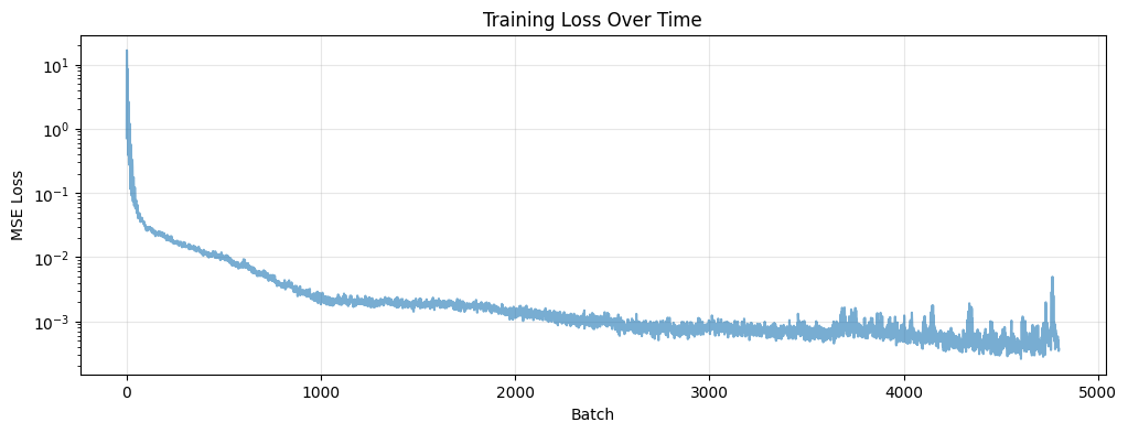
Training Loss Visualization

plt.figure(figsize=(12, 4))
plt.plot(loss_hist, alpha=0.6)
plt.title("Training Loss Over Time")
plt.xlabel("Batch")
plt.ylabel("MSE Loss")
plt.yscale('log')
plt.grid(True, alpha=0.3)
plt.show()

png

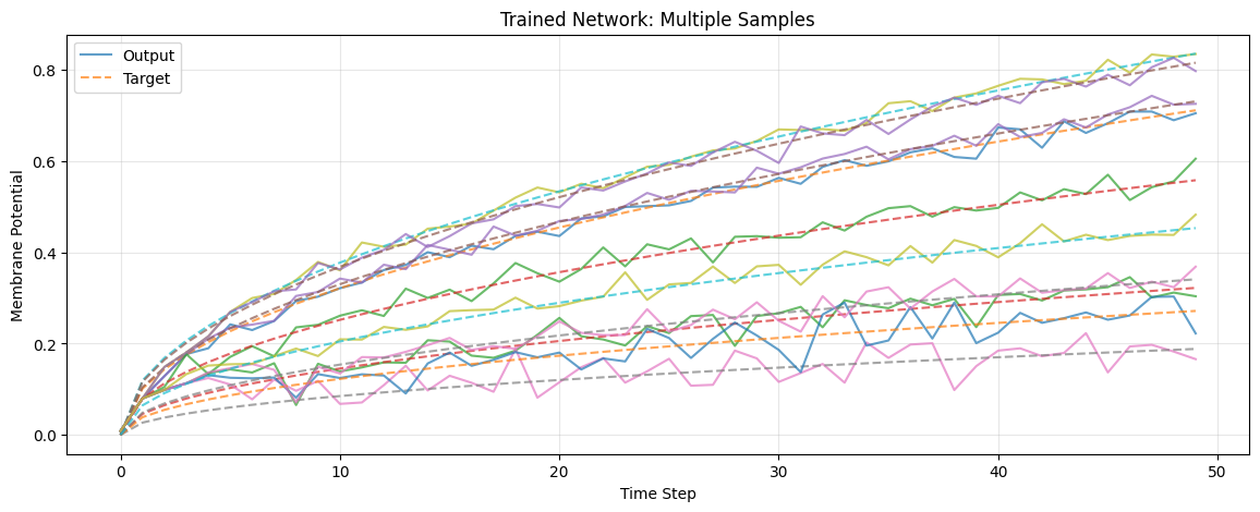
8. Evaluation and Results

Let's evaluate the trained network and visualize its performance.

# Switch to evaluation mode
model.eval()

# Get test batch
test_batch = iter(dataloader)
feature, label = next(test_batch)

# Evaluate without gradients
with torch.no_grad():
    feature = feature.to(device)
    label = label.to(device)
    spk, mem, spk_h = model(feature)

# Move to CPU for plotting
mem = mem.cpu()
label = label.cpu()
spk = spk.cpu()
spk_h = spk_h.cpu()

Visualize Multiple Predictions

plt.figure(figsize=(14, 5))
plt.title("Trained Network: Multiple Samples")
plt.xlabel("Time Step")
plt.ylabel("Membrane Potential")

# Plot multiple samples from the batch
num_samples_to_plot = min(10, batch_size)
for i in range(num_samples_to_plot):
    out_trace = mem[i, :, 0]
    target_trace = label[i, :, 0]

    # Only add labels for the first sample to avoid clutter
    plt.plot(out_trace, alpha=0.7, label="Output" if i == 0 else None)
    plt.plot(target_trace, "--", alpha=0.7, label="Target" if i == 0 else None)

plt.legend(loc="best")
plt.grid(True, alpha=0.3)
plt.show()

png

Detailed Single Sample Analysis

# Detailed view of a single sample
sample_idx = 0

fig, axes = plt.subplots(2, 1, figsize=(14, 8))

# Plot 1: Membrane potential
axes[0].plot(mem[sample_idx, :, 0], label="Output Membrane", linewidth=2)
axes[0].plot(label[sample_idx, :, 0], "--", label="Target", linewidth=2)
axes[0].set_title("Output Membrane Potential vs Target")
axes[0].set_xlabel("Time Step")
axes[0].set_ylabel("Membrane Potential")
axes[0].legend()
axes[0].grid(True, alpha=0.3)

# Plot 2: Hidden layer activity
axes[1].imshow(spk_h[sample_idx, :, :].T, aspect='auto', cmap='binary', interpolation='nearest')
axes[1].set_title("Hidden Layer Spike Activity")
axes[1].set_xlabel("Time Step")
axes[1].set_ylabel("Neuron Index")
axes[1].set_ylim([0, min(50, hidden_size)])  # Show first 50 neurons

plt.tight_layout()
plt.show()

print(f"\nFinal spike rate (output): {spk.mean().item():.4f}")
print(f"Final spike rate (hidden): {spk_h.mean().item():.4f}")

png

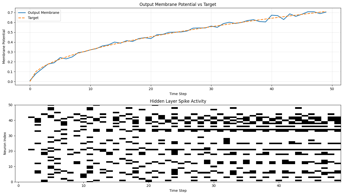
Final spike rate (output): 0.0000
Final spike rate (hidden): 0.2043

Performance Metrics

# Compute various metrics
mse = torch.nn.functional.mse_loss(mem[:, :, 0], label[:, :, 0])
mae = torch.nn.functional.l1_loss(mem[:, :, 0], label[:, :, 0])

# R² score
ss_res = torch.sum((label[:, :, 0] - mem[:, :, 0]) ** 2)
ss_tot = torch.sum((label[:, :, 0] - label[:, :, 0].mean()) ** 2)
r2_score = 1 - (ss_res / ss_tot)

print("\n=== Performance Metrics ===")
print(f"Mean Squared Error (MSE): {mse.item():.6f}")
print(f"Mean Absolute Error (MAE): {mae.item():.6f}")
print(f"R² Score: {r2_score.item():.6f}")

# Network activity metrics
print("\n=== Network Activity ===")
print(f"Output layer spike rate: {spk.mean().item():.4f}")
print(f"Hidden layer spike rate: {spk_h.mean().item():.4f}")
print(f"Active neurons (>0.1% spike rate): {(spk_h.mean(dim=[0,1]) > 0.001).sum().item()} / {hidden_size}")

=== Performance Metrics ===
Mean Squared Error (MSE): 0.000516
Mean Absolute Error (MAE): 0.016603
R² Score: 0.989620

=== Network Activity ===
Output layer spike rate: 0.0000
Hidden layer spike rate: 0.2043
Active neurons (>0.1% spike rate): 244 / 256

9. Summary: NWAVE vs snnTorch

Quick Comparison Table

Feature	NWAVE	snnTorch
Primary Purpose	Hardware deployment on Neuronova chips	SNN research and simulation
State Management	Automatic (internal to layers)	Manual (pass mem as argument)
Initialization	`prepare_net(model)` once	`mem = layer.init_leaky()` per layer
Data Format	`[B, T, N]` (batch-first)	`[T, B, N]` (time-first)
Layer Definition	`LIFSynapse` + `LIFLayer`	`nn.Linear` + `snn.Leaky`
Parameter Style	Physical (tau, dt, thresholds)	Abstract (beta)
Bias Control	Explicit `bias_learn`	Standard PyTorch
Reset Mechanism	Explicit parameter	Fixed per neuron type
PyTorch Integration	Standard conventions	SNN-specific conventions
Hardware Deployment	✅ Direct export to neuromorphic chips	❌ Simulation only

Migration Guide: snnTorch → NWAVE

Quick reference for porting existing code:

Aspect	snnTorch	NWAVE
Imports	`import snntorch as snn`	`from nwavesdk import LIFSynapse, LIFLayer, prepare_net`
Synapse	`nn.Linear(in, out)`	`LIFSynapse(in, out, use_bias=True, bias_learn=True)`
Neuron	`snn.Leaky(beta=0.9)`	`LIFLayer(n, taus=10e-3, thresholds=0.5, reset_mechanism="subtraction", dt=1e-3)`
Beta → Tau	`beta = 0.9`	`tau = -dt / log(beta) ≈ 9.5ms` (for dt=1ms)
Init State	`mem = lif.init_leaky()`	`prepare_net(model)`
Forward	`spk, mem = lif(cur, mem)`	`spk, mem = lif(cur)`
Data Shape	`[T, B, N]`	`[B, T, N]` (use `.permute(1,0,2)`)

Next Steps:

Try different neuron parameters (tau, threshold) to understand hardware constraints
Experiment with different network architectures (deeper, recurrent)
Explore the layer_topology="RC" option for recurrent connections
Check out Tutorial 2 for classification tasks with spike-based encoding
Learn about mismatch and quantization for Neuronova hardware deployment
Experiment with different reset mechanisms ("subtraction", "zero", "none")

Learn More:

Neuronova Technology - Hardware specifications and capabilities
NWAVE Documentation - Check your SDK installation for detailed API reference
Contact Neuronova for hardware deployment support and deployment tools