NWAVE Tutorial 3: Hardware-Aware Training with Frontend and Non-Idealities

Tutorial by Giuseppe Gentile and Marco Rasetto

Overview

This tutorial combines Frontend-based audio processing with hardware non-idealities to train robust, deployable networks using the Google Speech Commands dataset. We build on Tutorial 2 by adding:

Weight Quantization: Limited bit precision (5-bit default)
Device Mismatch: Variability in neuron parameters
Synaptic Variability: Weight noise from manufacturing variations (stddev)

Why Hardware-Aware Training?

When deploying to neuromorphic chips, models face real-world constraints that don't exist in software simulation. Training with these non-idealities produces networks that:

Are more robust to hardware imperfections
Maintain accuracy when deployed to physical chips
Better match real hardware behavior

What You'll Learn:

How to use Frontend with quantization and mismatch
How to enable quantization in HWSynapse layers
How to simulate synaptic weight variability (stddev)
How to apply device mismatch to HWLayer neurons
How to train with hardware constraint losses (topology_loss, weight_magnitude_loss)
How to compare ideal vs. non-ideal training
Best practices for hardware-aware training

1. Setup and Imports

!pip -q install torchaudio

import os
import shutil
import random
import numpy as np
import torch
import torch.nn as nn
from torch.utils.data import DataLoader, random_split
import torchaudio
import matplotlib.pyplot as plt

# ============================================
# NWAVE IMPORTS FOR HARDWARE-READY MODELS
# ============================================
from nwavesdk.layers import HWSynapse, HWLayer, Frontend, prepare_net
from nwavesdk.metrics import get_chip_consumption
from nwavesdk.loss import topology_loss, weight_magnitude_loss
from nwavesdk.surrogate import fast_sigmoid

# Set random seeds for reproducibility
torch.manual_seed(7)
np.random.seed(7)
random.seed(7)

device = "cpu"
print("Setup complete!")

Setup complete!

# Display hardware parameter defaults
print("=== Empiric Hardware Parameters ===\n")
print(f"  w_min: -0.9")
print(f"  w_max:  0.9")

print(f"  stddv (variability): 4")

print("\nThese parameters model real hardware characteristics of Neuronova chips.")

=== Empiric Hardware Parameters ===

  w_min: -0.9
  w_max:  0.9
  stddv (variability): 4

These parameters model real hardware characteristics of Neuronova chips.

NWAVE Function Reference

This section documents all the NWAVE functions and classes used in this tutorial.

Layers

`Frontend(nb_inputs, quantization_bits=None, stddev=None, init=xavier_uniform_, lif_threshold=1.0)`

Simulates the analog frontend of Neuronova's hardware with optional non-idealities.

Parameters:

Parameter	Type	Description
`nb_inputs`	int	Number of input channels/filters
`quantization_bits`	int, optional	Bits for weight quantization (None = no quantization)
`stddev`	float, optional	Std dev for synaptic mismatch noise simulation
`init`	callable	Weight initialization function
`lif_threshold`	float	Threshold for weight initialization scaling

`HWSynapse(nb_inputs, nb_outputs, quantization_bit=None, stddev=None, ...)`

Hardware-realistic dense synaptic connections with optional quantization and mismatch.

Parameters:

Parameter	Type	Description
`nb_inputs`	int	Number of input neurons
`nb_outputs`	int	Number of output neurons
`quantization_bit`	int, optional	Bits for weight quantization
`stddev`	float, optional	Std dev for synaptic mismatch noise

`HWLayer(n_neurons, taus, dt, ileak_mismatch=False, ...)`

Hardware spiking neuron layer with optional device mismatch.

Parameters:

Parameter	Type	Description
`n_neurons`	int	Number of neurons in the layer
`taus`	float/Tensor	Membrane time constants
`dt`	float	Integration timestep in seconds
`ileak_mismatch`	bool	Enable mismatch in leak current (default: False)

Loss Functions

`topology_loss(model, lam)`

Regularizer that encourages sign alignment within groups of 5 neurons.

`weight_magnitude_loss(model, limit=0.9)`

L2 penalty for weights exceeding a magnitude limit.

2. Dataset and Preprocessing

We use the Google Speech Commands dataset, a popular benchmark for keyword spotting.

Available words: yes, no, up, down, left, right, on, off, stop, go, and more.

Task: Binary classification between 2 selected words.

Configuration: You can change WORD_1 and WORD_2 below to use any pair of words.

# ============================================
# CONFIGURATION: Choose your 2 words
# ============================================
# Available words in Speech Commands v0.02:
# yes, no, up, down, left, right, on, off, stop, go,
# zero, one, two, three, four, five, six, seven, eight, nine,
# bed, bird, cat, dog, happy, house, marvin, sheila, tree, wow

WORD_1 = "yes"  # Class 0
WORD_2 = "no"   # Class 1

# Audio parameters
SAMPLE_RATE = 16000  # Speech Commands native sample rate
RECORDING_DURATION_S = 1.0  # Each clip is 1 second

print(f"Training binary classifier: '{WORD_1}' (class 0) vs '{WORD_2}' (class 1)")

Training binary classifier: 'yes' (class 0) vs 'no' (class 1)

from torchaudio.datasets import SPEECHCOMMANDS

# Download Speech Commands dataset
os.makedirs("data", exist_ok=True)

class SubsetSpeechCommands(SPEECHCOMMANDS):
    """Speech Commands dataset filtered to specific words."""
    def __init__(self, root, subset, words, download=True):
        super().__init__(root, download=download, subset=subset)
        self.words = words
        # Filter to only include specified words
        self._walker = [
            item for item in self._walker 
            if os.path.basename(os.path.dirname(item)) in words
        ]

# Load training and validation subsets
print(f"Downloading Speech Commands dataset (this may take a few minutes)...")
train_dataset = SubsetSpeechCommands("data", subset="training", words=[WORD_1, WORD_2])
val_dataset = SubsetSpeechCommands("data", subset="validation", words=[WORD_1, WORD_2])

print(f"\nDataset loaded:")
print(f"  Training samples: {len(train_dataset)}")
print(f"  Validation samples: {len(val_dataset)}")

Downloading Speech Commands dataset (this may take a few minutes)...

Dataset loaded:
  Training samples: 6358
  Validation samples: 803

import scipy.io.wavfile as wavfile

# Prepare data directory structure for NWaveDataGen
# NWaveDataGen expects: data_parent/class_name/*.wav

target_dir = "data_for_nwave_commands"
word1_dir = os.path.join(target_dir, WORD_1)
word2_dir = os.path.join(target_dir, WORD_2)

# Clean and create directories
if os.path.exists(target_dir):
    shutil.rmtree(target_dir)
os.makedirs(word1_dir, exist_ok=True)
os.makedirs(word2_dir, exist_ok=True)

def save_dataset_to_folders(dataset, word1_dir, word2_dir, word1, word2, prefix=""):
    """Save dataset samples to class folders as WAV files."""
    counts = {word1: 0, word2: 0}

    for i, (waveform, sample_rate, label, speaker_id, utterance_num) in enumerate(dataset):
        # Determine output directory based on label
        if label == word1:
            out_dir = word1_dir
        elif label == word2:
            out_dir = word2_dir
        else:
            continue

        # Convert to numpy and ensure correct format
        audio = waveform.squeeze().numpy()

        # Pad or trim to exactly 1 second
        target_length = sample_rate  # 1 second
        if len(audio) < target_length:
            audio = np.pad(audio, (0, target_length - len(audio)))
        else:
            audio = audio[:target_length]

        # Convert to int16 for WAV file (scipy.io.wavfile format)
        audio_int16 = (audio * 32767).astype(np.int16)

        # Save file
        filename = f"{prefix}{label}_{speaker_id}_{utterance_num}_{i}.wav"
        filepath = os.path.join(out_dir, filename)
        wavfile.write(filepath, sample_rate, audio_int16)
        counts[label] += 1

    return counts

# Save training data
print("Preparing training data...")
train_counts = save_dataset_to_folders(
    train_dataset, word1_dir, word2_dir, WORD_1, WORD_2, prefix="train_"
)

# Save validation data
print("Preparing validation data...")
val_counts = save_dataset_to_folders(
    val_dataset, word1_dir, word2_dir, WORD_1, WORD_2, prefix="val_"
)

print(f"\nData prepared in '{target_dir}':")
print(f"  {WORD_1}/: {train_counts[WORD_1] + val_counts[WORD_1]} files")
print(f"  {WORD_2}/: {train_counts[WORD_2] + val_counts[WORD_2]} files")

Preparing training data...
Preparing validation data...

Data prepared in 'data_for_nwave_commands':
  yes/: 3625 files
  no/: 3536 files

from nwavesdk import NWaveDataGen, NWaveDataloaderConfig 

data_config = NWaveDataloaderConfig(
    batch_size=16,
    val_split=0.15,
    test_split=0.,
    random_state=123,
    num_workers=4,
    shuffle_train=True,
)

# Create data generator with hardware filterbank
dm = NWaveDataGen(
    data_parent=target_dir,
    sample_rate=SAMPLE_RATE,
    recording_duration_s=RECORDING_DURATION_S,
    sim_time_s=8e-3,  # 8ms time bins
    dataloader_config=data_config,
    task="classification",
    return_filename=True
)

loaders = dm.dataloaders()
train_loader = loaders["train"]
val_loader = loaders["val"]

# Get number of filter channels from first batch
x, y, fn = next(iter(train_loader))
N_CHANNELS = x.shape[2]
print(f"\nInput shape: {x.shape} (batch, timesteps, channels)")
print(f"Number of filter channels: {N_CHANNELS}")
print(f"\nDataset split: {len(train_loader.dataset)} train, {len(val_loader.dataset)} validation")

2026-02-05 16:09:06,556 - root - WARNING - Using 13 valid freqs out of 16 for sr=16000Hz (Nyquist=8000.0Hz).
Classes (loading wavs): 100%|██████████| 2/2 [00:01<00:00,  1.37it/s]
Filtering no: 100%|██████████| 3536/3536 [00:22<00:00, 156.32it/s]
Filtering yes: 100%|██████████| 3625/3625 [00:22<00:00, 158.25it/s]



Input shape: torch.Size([16, 125, 13]) (batch, timesteps, channels)
Number of filter channels: 13

Dataset split: 6087 train, 1074 validation

# # (Optional) Save/Load dataloader
torch.save(train_loader, "train_commands.pt")
torch.save(val_loader, "val_commands.pt")

train_loader = torch.load("train_commands.pt", weights_only=False)
val_loader = torch.load("val_commands.pt", weights_only=False)

3. Understanding Hardware Non-Idealities

Before building our models, let's understand the three types of non-idealities we'll simulate:

3.1 Weight Quantization

Real hardware uses limited bit precision for weights (typically 5-bit). This means weights are discretized to a small set of values instead of continuous 32-bit floats.

In NWAVE: Set quantization_bits parameter in Frontend and HWSynapse

3.2 Synaptic Variability (stddev)

Manufacturing variations cause slight differences in synaptic weights across the chip. This is modeled as Gaussian noise added to the charge transfer function.

In NWAVE: Set stddev parameter in HWSynapse (default: 4.0)

Warning

Do NOT use stddev on Frontend - it can cause numerical instability due to small frontend weights.

3.3 Device Mismatch

Individual neurons have slight variations in their leak current due to manufacturing imperfections, affecting membrane dynamics.

In NWAVE: Set ileak_mismatch=True in HWLayer (core layers only)

Warning

Avoid ileak_mismatch on frontend HWLayer for training stability.

Training Strategy

We'll train three models to compare:

Ideal Model: No non-idealities (baseline)
Quantized Model: With quantization only
Full Hardware Model: Quantization on all layers + stddev/mismatch on core layers only

Hardware Constraints and Custom Losses

When deploying models to the Neuronova chip, several hardware constraints must be respected during training.

1. Weight Magnitude Constraint

Synaptic weights are stored in analog memories with a limited dynamic range.

Solution: weight_magnitude_loss(model, limit=0.9) penalizes weights exceeding the limit.

2. Sign Alignment Constraint (Topology Loss)

Due to hardware architecture, groups of 5 contiguous synapses must share the same sign.

Solution: topology_loss(model, lam) encourages sign alignment within groups.

3. Firing Rate Regularization

Ensures neurons fire at a target rate for optimal power consumption and information transfer.

Combined Loss Function

loss = loss_task + topology_loss(model, lam=0.05) + weight_magnitude_loss(model) + fr_loss(spikes)

4. Hardware-Ready SNN Model with Non-Idealities

We build a 3-layer spiking network using Frontend, HWSynapse, and HWLayer with configurable non-idealities:

Architecture:

Input [B, T, C] → Frontend (diagonal) → HWLayer [B, T, C]
                                              ↓
                    HWSynapse (dense) → HWLayer [B, T, 64] (hidden)
                                              ↓
                    HWSynapse (dense) → HWLayer [B, T, 2] (output)

class FrontendNet(nn.Module):
    """Frontend layer with configurable non-idealities.

    Args:
        dt: Simulation timestep
        n_channels: Number of input channels
        quantization_bits: Bit precision (None = full precision)
        stddev: Synaptic variability (None = no variability)
        ileak_mismatch: Enable neuron mismatch
    """
    def __init__(self, dt=8e-3, n_channels=16, 
                 quantization_bits=None, stddev=None, ileak_mismatch=False):
        super().__init__()

        # Frontend synapse with optional non-idealities
        self.frontend_syn = Frontend(
            nb_inputs=n_channels,
            quantization_bits=quantization_bits,
            stddev=stddev,
            init=lambda w: nn.init.normal_(w, 0.1, 0.01),
        )

        # LIF neurons with optional mismatch
        self.hw1 = HWLayer(
            n_neurons=n_channels, 
            taus=10e-3,
            dt=dt, 
            ileak_mismatch=ileak_mismatch,
            spike_grad=fast_sigmoid(slope=25.0)
        )

    def forward(self, x):
        B, T, _ = x.shape

        mem_trace = []
        spk_trace = []
        cur_trace = []

        prepare_net(self)

        for t in range(T):
            cur1 = self.frontend_syn(x[:, t, :])
            cur_trace.append(cur1)
            spk1, mem1 = self.hw1(cur1)
            mem_trace.append(mem1)
            spk_trace.append(spk1)

        mem_trace = torch.stack(mem_trace, dim=1)
        spk_trace = torch.stack(spk_trace, dim=1)
        self.cur_trace = torch.stack(cur_trace, dim=1)

        return spk_trace


class HWSNN(nn.Module):
    """Hardware-ready SNN core with configurable non-idealities.

    Args:
        n_channels: Number of input channels
        num_classes: Number of output classes
        hidden_size: Number of hidden neurons
        dt: Simulation timestep
        quantization_bit: Bit precision (None = full precision) - NOTE: singular for HWSynapse
        stddev: Synaptic variability (None = no variability)
        ileak_mismatch: Enable neuron mismatch
    """
    def __init__(self, n_channels, num_classes=2, hidden_size=32, dt=8e-3,
                 quantization_bit=None, stddev=None, ileak_mismatch=False):
        super().__init__()
        self.hidden_size = hidden_size
        self.num_classes = num_classes
        self.dt = dt

        taus = 64e-3

        # Hidden layer with non-idealities
        self.syn_hidden = HWSynapse(
            n_channels, hidden_size,
            quantization_bit=quantization_bit,
            stddev=stddev,
            init=lambda w: nn.init.normal_(w, 0.1, 0.3)
        )
        self.hw_hidden = HWLayer(
            n_neurons=hidden_size, 
            taus=taus, 
            dt=dt,
            ileak_mismatch=ileak_mismatch,
            spike_grad=fast_sigmoid(slope=25.0)
        )

        # Output layer with non-idealities
        self.syn_out = HWSynapse(
            hidden_size, num_classes,
            quantization_bit=quantization_bit,
            stddev=stddev,
            init=lambda w: nn.init.normal_(w, 0.1, 0.3),
        )
        self.hw_out = HWLayer(
            n_neurons=num_classes, 
            taus=taus, 
            dt=dt,
            ileak_mismatch=ileak_mismatch,
            spike_grad=fast_sigmoid(slope=25.0)
        )

    def forward(self, x):
        B, T, _ = x.shape

        spk_hidden_trace = []
        spk_out_trace = []

        prepare_net(self)

        for t in range(T):
            cur_hidden = self.syn_hidden(x[:, t, :])
            spk_hidden, mem_hidden = self.hw_hidden(cur_hidden)
            spk_hidden_trace.append(spk_hidden)

            cur_out = self.syn_out(spk_hidden)
            spk_out, mem_out = self.hw_out(cur_out)
            spk_out_trace.append(spk_out)

        self.spk_hidden_trace = torch.stack(spk_hidden_trace, dim=1)
        self.spk_out_trace = torch.stack(spk_out_trace, dim=1)

        return self.spk_out_trace

# ============================================
# CREATE THREE MODEL VARIANTS
# ============================================
torch.manual_seed(42)

HIDDEN_SIZE = 64

print("\n=== Creating Three Model Variants ===\n")

# Model 1: Ideal (no non-idealities)
# Note: Frontend uses quantization_bits, HWSynapse uses quantization_bit
frontend_ideal = FrontendNet(
    n_channels=N_CHANNELS,
    quantization_bits=None,
    stddev=None,
    ileak_mismatch=False
).to(device)
core_ideal = HWSNN(
    n_channels=N_CHANNELS,
    hidden_size=HIDDEN_SIZE,
    quantization_bit=None,  # singular for HWSynapse
    stddev=None,
    ileak_mismatch=False
).to(device)
model_ideal = nn.Sequential(frontend_ideal, core_ideal)
print("1. Ideal Model (baseline - no non-idealities)")
print(f"   - Full precision weights (32-bit)")
print(f"   - No synaptic variability")
print(f"   - No device mismatch")

# Model 2: Quantized only
frontend_quant = FrontendNet(
    n_channels=N_CHANNELS,
    quantization_bits=5,
    stddev=None,
    ileak_mismatch=False
).to(device)
core_quant = HWSNN(
    n_channels=N_CHANNELS,
    hidden_size=HIDDEN_SIZE,
    quantization_bit=5,  # singular for HWSynapse
    stddev=None,
    ileak_mismatch=False
).to(device)
model_quant = nn.Sequential(frontend_quant, core_quant)
print("\n2. Quantized Model")
print(f"   - 5-bit quantized weights")
print(f"   - No synaptic variability")
print(f"   - No device mismatch")

# Model 3: Full hardware (all non-idealities on core, quantization only on frontend)
# NOTE: Frontend uses quantization but NOT stddev/mismatch, as these can cause
# numerical instability with small frontend weights. Core layers use full non-idealities.
frontend_hw = FrontendNet(
    n_channels=N_CHANNELS,
    quantization_bits=5,    # Quantization OK on frontend
    stddev=None,            # No stddev on frontend for numerical stability
    ileak_mismatch=False    # No mismatch on frontend for numerical stability
).to(device)
core_hw = HWSNN(
    n_channels=N_CHANNELS,
    hidden_size=HIDDEN_SIZE,
    quantization_bit=5,     # Full quantization on core
    stddev=4.0,             # Full stddev on core layers
    ileak_mismatch=True     # Full mismatch on core layers
).to(device)
model_hw = nn.Sequential(frontend_hw, core_hw)
print("\n3. Full Hardware Model (most realistic)")
print(f"   - 5-bit quantized weights (frontend + core)")
print(f"   - Synaptic variability (stddev=4.0) on CORE layers only")
print(f"   - Device mismatch on CORE layers only")
print(f"   - (Frontend stddev/mismatch disabled for numerical stability)")

print("\n" + "="*60)
print(f"\nTotal parameters per model: {sum(p.numel() for p in model_ideal.parameters()):,}")

=== Creating Three Model Variants ===

1. Ideal Model (baseline - no non-idealities)
   - Full precision weights (32-bit)
   - No synaptic variability
   - No device mismatch

2. Quantized Model
   - 5-bit quantized weights
   - No synaptic variability
   - No device mismatch

3. Full Hardware Model (most realistic)
   - 5-bit quantized weights (frontend + core)
   - Synaptic variability (stddev=4.0) on CORE layers only
   - Device mismatch on CORE layers only
   - (Frontend stddev/mismatch disabled for numerical stability)

============================================================

Total parameters per model: 973


/tmp/ipykernel_3112675/3318570476.py:16: UserWarning: Frontend on chip uses 16 filters. Using a different amount of neurons 13 is allowed but not respecting the chip constraints.
  self.frontend_syn = Frontend(

5. Training All Three Models with Hardware Losses

We train all three models with the full loss function including:

CrossEntropyLoss: Main classification loss
topology_loss: Sign alignment constraint
weight_magnitude_loss: Weight clipping constraint
firing_rate_target_mse_loss: Firing rate regularization

from nwavesdk.loss import firing_rate_target_mse_loss
from nwavesdk.metrics import accuracy

def evaluate(model, loader):
    """Evaluate model accuracy on a dataloader."""
    model.eval()
    correct = 0
    total = 0

    with torch.no_grad():
        for specs, labels, fn in loader:
            specs = specs.to(device)
            labels = labels.to(device)

            spike_traces = model(specs)
            correct += accuracy(spike_traces, labels)
            total += 1

    return correct / max(total, 1)


def train_model(model, frontend, core_net, name, epochs=50, 
                lr_frontend=1e-5, lr_core=1e-3,
                lam_topology=0.05, lam_fr=10, target_fr=0.30):
    """Train a model with hardware constraint losses."""

    criterion = nn.CrossEntropyLoss()
    optimizer = torch.optim.Adam([
        {'params': frontend.parameters(), 'lr': lr_frontend},
        {'params': core_net.parameters(), 'lr': lr_core},
    ])

    history = {
        'train_loss': [], 'loss_main': [], 'train_acc': [], 'val_acc': [],
        'fr_n0': [], 'fr_n1': []
    }

    best_acc = 0.0
    best_state = None

    print(f"\n{'='*60}")
    print(f"Training {name}")
    print(f"{'='*60}")
    print(f"Frontend LR: {lr_frontend} | Core LR: {lr_core}")
    print(f"Topology λ: {lam_topology} | FR λ: {lam_fr} | Target FR: {target_fr}\n")
    print(f"{'Epoch':<6} | {'Loss':<7} | {'Train':<7} | {'Val':<7} | {'Best':<5}")
    print("-" * 50)

    for epoch in range(1, epochs + 1):
        model.train()
        running_loss, running_main = 0.0, 0.0
        train_correct, train_total = 0, 0

        for specs, labels, fn in train_loader:
            specs, labels = specs.to(device), labels.to(device)

            optimizer.zero_grad()

            spike_counts = model(specs)
            logits = spike_counts.sum(dim=1)

            # Combined loss with hardware constraints
            loss_main = criterion(logits, labels)
            loss_topo = topology_loss(core_net, lam=lam_topology)
            loss_mag = weight_magnitude_loss(core_net)
            loss_fr = firing_rate_target_mse_loss(spikes_list = [spike_counts], offsets = [target_fr], multipliers = [lam_fr])

            loss = loss_main + loss_fr + loss_topo + loss_mag
            loss.backward()

            torch.nn.utils.clip_grad_norm_(model.parameters(), max_norm=0.5)
            optimizer.step()

            preds = logits.argmax(dim=1)
            train_correct += (preds == labels).sum().item()
            train_total += labels.size(0)

            batch_size = labels.size(0)
            running_loss += loss.item() * batch_size
            running_main += loss_main.item() * batch_size

        # Epoch statistics
        n_samples = len(train_loader.dataset)
        epoch_loss = running_loss / n_samples
        train_acc = train_correct / train_total
        val_acc = evaluate(model, val_loader)

        history['train_loss'].append(epoch_loss)
        history['train_acc'].append(train_acc)
        history['val_acc'].append(val_acc)

        # Track best model
        is_best = ""
        if val_acc > best_acc:
            best_acc = val_acc
            best_state = {k: v.clone() for k, v in model.state_dict().items()}
            is_best = "★"

        if epoch % 10 == 0 or epoch == 1 or is_best:
            print(f"{epoch:<6} | {epoch_loss:<7.4f} | {train_acc:<7.1%} | {val_acc:<7.1%} | {is_best}")

    # Restore best model
    if best_state is not None:
        model.load_state_dict(best_state)

    print(f"\nBest validation accuracy: {best_acc:.1%}")

    return history, best_acc

# ============================================
# TRAIN ALL THREE MODELS
# ============================================
print("="*70)
print(f"TRAINING COMPARISON: Ideal vs Quantized vs Full Hardware")
print(f"Task: {WORD_1} vs {WORD_2}")
print("="*70)
print("\nNote: Full Hardware model may require more epochs due to:")
print("  1. Quantization (5-bit) limits weight precision")
print("  2. Synaptic noise (stddev=4.0) adds stochastic perturbations")
print("  3. Device mismatch creates neuron-to-neuron variability")

EPOCHS = 50

# Train Ideal Model
history_ideal, best_ideal = train_model(
    model_ideal, frontend_ideal, core_ideal,
    "Ideal Model", epochs=EPOCHS
)

# # Train Quantized Model
history_quant, best_quant = train_model(
    model_quant, frontend_quant, core_quant,
    "Quantized Model", epochs=EPOCHS
)

# Train Full Hardware Model
history_hw, best_hw = train_model(
    model_hw, frontend_hw, core_hw,
    "Full Hardware Model", epochs=EPOCHS
)

print("\n" + "="*70)
print("TRAINING COMPLETED")
print("="*70)
print(f"\nFinal Results:")
print(f"  Ideal Model:       {best_ideal:.1%}")
print(f"  Quantized Model:   {best_quant:.1%}")
print(f"  Full HW Model:     {best_hw:.1%}")

======================================================================
TRAINING COMPARISON: Ideal vs Quantized vs Full Hardware
Task: yes vs no
======================================================================

Note: Full Hardware model may require more epochs due to:
  1. Quantization (5-bit) limits weight precision
  2. Synaptic noise (stddev=4.0) adds stochastic perturbations
  3. Device mismatch creates neuron-to-neuron variability

============================================================
Training Ideal Model
============================================================
Frontend LR: 1e-05 | Core LR: 0.001
Topology λ: 0.05 | FR λ: 10 | Target FR: 0.3

Epoch  | Loss    | Train   | Val     | Best 
--------------------------------------------------
1      | 5.1852  | 65.9%   | 63.8%   | ★
2      | 2.5954  | 71.9%   | 83.9%   | ★
5      | 1.4695  | 80.7%   | 85.0%   | ★
8      | 0.8060  | 84.8%   | 86.4%   | ★
10     | 0.8370  | 85.1%   | 85.5%   | 
14     | 0.8108  | 83.9%   | 87.0%   | ★
16     | 0.7551  | 85.7%   | 87.3%   | ★
20     | 0.7252  | 86.5%   | 87.0%   | 
23     | 0.8157  | 86.1%   | 87.6%   | ★
26     | 0.7313  | 86.4%   | 88.4%   | ★
30     | 0.7585  | 87.1%   | 87.6%   | 
34     | 0.7773  | 87.3%   | 89.3%   | ★
40     | 0.6797  | 87.4%   | 85.3%   | 
47     | 0.8368  | 86.7%   | 89.4%   | ★
50     | 0.7038  | 86.5%   | 88.1%   |

Best validation accuracy: 89.4%

============================================================
Training Quantized Model
============================================================
Frontend LR: 1e-05 | Core LR: 0.001
Topology λ: 0.05 | FR λ: 10 | Target FR: 0.3

Epoch  | Loss    | Train   | Val     | Best 
--------------------------------------------------
1      | 4.4533  | 67.8%   | 72.8%   | ★
2      | 1.5798  | 73.1%   | 76.3%   | ★
3      | 1.5065  | 77.0%   | 85.5%   | ★
4      | 0.7358  | 85.8%   | 86.3%   | ★
7      | 0.7231  | 86.6%   | 88.4%   | ★
8      | 0.6959  | 86.9%   | 89.3%   | ★
10     | 0.6096  | 88.4%   | 88.7%   | 
15     | 1.0314  | 85.4%   | 89.6%   | ★
20     | 0.9447  | 86.6%   | 89.5%   | 
30     | 0.8086  | 87.2%   | 65.1%   | 
32     | 0.9850  | 87.4%   | 89.9%   | ★
40     | 0.8696  | 86.7%   | 89.6%   | 
50     | 0.7580  | 87.2%   | 87.4%   |

Best validation accuracy: 89.9%

============================================================
Training Full Hardware Model
============================================================
Frontend LR: 1e-05 | Core LR: 0.001
Topology λ: 0.05 | FR λ: 10 | Target FR: 0.3

Epoch  | Loss    | Train   | Val     | Best 
--------------------------------------------------


2026-02-05 16:51:32,070 - root - INFO - Synapse mismatch at stddev = 4.0 has now been enabled
2026-02-05 16:51:32,076 - root - INFO - Synapse mismatch at stddev = 4.0 has now been enabled


1      | 8.3500  | 61.7%   | 67.8%   | ★
3      | 5.0313  | 68.2%   | 71.0%   | ★
5      | 3.3826  | 72.3%   | 75.6%   | ★
6      | 2.4607  | 76.1%   | 78.5%   | ★
10     | 1.7054  | 79.5%   | 71.3%   | 
11     | 1.6297  | 79.8%   | 81.2%   | ★
13     | 1.4141  | 81.2%   | 83.1%   | ★
15     | 1.2643  | 82.0%   | 85.6%   | ★
20     | 1.1177  | 84.4%   | 84.0%   | 
27     | 1.1031  | 84.1%   | 85.7%   | ★
29     | 1.0791  | 84.1%   | 85.8%   | ★
30     | 0.9234  | 85.0%   | 80.2%   | 
40     | 0.9565  | 85.4%   | 86.0%   | ★
45     | 0.9451  | 85.1%   | 88.3%   | ★
50     | 0.8918  | 85.1%   | 82.4%   |

Best validation accuracy: 88.3%

======================================================================
TRAINING COMPLETED
======================================================================

Final Results:
  Ideal Model:       89.4%
  Quantized Model:   89.9%
  Full HW Model:     88.3%

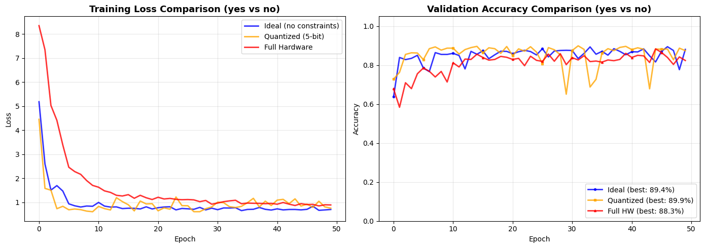
6. Comparison Plots

Let's visualize how hardware non-idealities affect training convergence and final accuracy.

fig, axes = plt.subplots(1, 2, figsize=(14, 5))

# Plot 1: Training Loss Comparison
axes[0].plot(history_ideal['train_loss'], linewidth=2, label='Ideal (no constraints)', color='blue', alpha=0.8)
axes[0].plot(history_quant['train_loss'], linewidth=2, label='Quantized (5-bit)', color='orange', alpha=0.8)
axes[0].plot(history_hw['train_loss'], linewidth=2, label='Full Hardware', color='red', alpha=0.8)
axes[0].set_title(f'Training Loss Comparison ({WORD_1} vs {WORD_2})', fontsize=13, fontweight='bold')
axes[0].set_xlabel('Epoch')
axes[0].set_ylabel('Loss')
axes[0].legend(loc='upper right')
axes[0].grid(True, alpha=0.3)

# Plot 2: Validation Accuracy Comparison
axes[1].plot(history_ideal['val_acc'], linewidth=2, marker='o', markersize=3, markevery=5,
             label=f'Ideal (best: {best_ideal:.1%})', color='blue', alpha=0.8)
axes[1].plot(history_quant['val_acc'], linewidth=2, marker='s', markersize=3, markevery=5,
             label=f'Quantized (best: {best_quant:.1%})', color='orange', alpha=0.8)
axes[1].plot(history_hw['val_acc'], linewidth=2, marker='^', markersize=3, markevery=5,
             label=f'Full HW (best: {best_hw:.1%})', color='red', alpha=0.8)
axes[1].set_title(f'Validation Accuracy Comparison ({WORD_1} vs {WORD_2})', fontsize=13, fontweight='bold')
axes[1].set_xlabel('Epoch')
axes[1].set_ylabel('Accuracy')
axes[1].set_ylim(0, 1.05)
axes[1].legend(loc='lower right')
axes[1].grid(True, alpha=0.3)

plt.tight_layout()
plt.show()

png

7. Hardware Power Consumption Analysis

Let's estimate power consumption for the Full Hardware model.

# Run inference and collect spike data for power analysis
model_hw.eval()
all_spk_hidden = []
all_spk_output = []

with torch.no_grad():
    for specs, labels, fn in val_loader:
        specs = specs.to(device)
        spk_frontend = frontend_hw(specs)
        spk_output = core_hw(spk_frontend)
        all_spk_hidden.append(core_hw.spk_hidden_trace)
        all_spk_output.append(spk_output)

all_spk_hidden = torch.cat(all_spk_hidden, dim=0)
all_spk_output = torch.cat(all_spk_output, dim=0)

# Create flat model with core HW layers
hw_model = nn.Sequential(
    core_hw.syn_hidden,
    core_hw.hw_hidden,
    core_hw.syn_out,
    core_hw.hw_out,
)

spks = [all_spk_hidden, all_spk_output]
total_power = get_chip_consumption(hw_model, spks, dt=core_hw.dt)

n_timesteps = all_spk_hidden.shape[1]
energy_per_inference = total_power * n_timesteps * core_hw.dt

print("="*50)
print(f"HARDWARE POWER CONSUMPTION ({WORD_1} vs {WORD_2})")
print("="*50)
print(f"Total power:           {total_power*1e6:.3f} µW")
print(f"Energy per inference:  {energy_per_inference*1e9:.3f} nJ")
print(f"\nSpike rates:")
print(f"  Hidden layer: {all_spk_hidden.mean().item()*100:.1f}%")
print(f"  Output layer: {all_spk_output.mean().item()*100:.1f}%")

==================================================
HARDWARE POWER CONSUMPTION (yes vs no)
==================================================
Total power:           0.013 µW
Energy per inference:  13.370 nJ

Spike rates:
  Hidden layer: 40.3%
  Output layer: 30.7%

8. Saving and Loading Models

NWAVE models are fully compatible with PyTorch's save/load mechanism.

# Save the Full Hardware model (recommended for deployment)
model_filename = f'hwsnn_fullhw_{WORD_1}_{WORD_2}.pth'
torch.save(model_hw.state_dict(), model_filename)
print(f"Full HW model saved to '{model_filename}'")

# To load:
print(f"\nTo load the model:")
print(f"""```python
# Frontend: quantization only (no stddev/mismatch for stability)
loaded_frontend = FrontendNet(
    n_channels={N_CHANNELS}, 
    quantization_bits=5, 
    stddev=None,           # No stddev on frontend!
    ileak_mismatch=False   # No mismatch on frontend!
)
# Core: full non-idealities
loaded_core = HWSNN(
    n_channels={N_CHANNELS}, 
    hidden_size={HIDDEN_SIZE}, 
    quantization_bit=5, 
    stddev=4.0,            # Full stddev on core
    ileak_mismatch=True    # Full mismatch on core
)
loaded_model = nn.Sequential(loaded_frontend, loaded_core)
loaded_model.load_state_dict(torch.load('{model_filename}'))
```""")

Full HW model saved to 'hwsnn_fullhw_yes_no.pth'

To load the model:
```python
# Frontend: quantization only (no stddev/mismatch for stability)
loaded_frontend = FrontendNet(
    n_channels=13, 
    quantization_bits=5, 
    stddev=None,           # No stddev on frontend!
    ileak_mismatch=False   # No mismatch on frontend!
)
# Core: full non-idealities
loaded_core = HWSNN(
    n_channels=13, 
    hidden_size=64, 
    quantization_bit=5, 
    stddev=4.0,            # Full stddev on core
    ileak_mismatch=True    # Full mismatch on core
)
loaded_model = nn.Sequential(loaded_frontend, loaded_core)
loaded_model.load_state_dict(torch.load('hwsnn_fullhw_yes_no.pth'))
```

9. Best Practices for Hardware-Aware Training

======================================================================
BEST PRACTICES FOR HARDWARE-AWARE TRAINING
======================================================================

1. QUANTIZATION
   ✓ Enable in BOTH Frontend and HWSynapse for deployment
   ✓ Use 5-bit (default) for Neuronova chips
   ✓ NOTE: Different parameter names!

   Example:
   Frontend(nb_inputs, quantization_bits=5)    # plural
   HWSynapse(in_features, out_features, quantization_bit=5)  # singular

2. SYNAPTIC VARIABILITY (stddev parameter)
   ✓ Enable stddev on HWSynapse layers (core network)
   ⚠ AVOID stddev on Frontend - causes numerical instability!
   ✓ Use default stddev=4.0 for realistic simulation

   Example:
   Frontend(nb_inputs, stddev=None)  # Keep None for stability!
   HWSynapse(in_features, out_features, stddev=4.0)

3. DEVICE MISMATCH (ileak_mismatch parameter)
   ✓ Enable on HWLayer instances in core network
   ⚠ AVOID on Frontend layer - can cause gradient issues

   Example:
   # Frontend layer
   HWLayer(n_neurons, taus, dt, ileak_mismatch=False)  # Frontend
   # Core layers  
   HWLayer(n_neurons, taus, dt, ileak_mismatch=True)   # Core

4. HARDWARE CONSTRAINT LOSSES
   ✓ Use topology_loss() for sign alignment
   ✓ Use weight_magnitude_loss() for weight clipping
   ✓ Use fr_loss() for firing rate regularization

   Example:
   loss = loss_main + topology_loss(model, lam=0.05) + weight_magnitude_loss(model) + fr_loss(spk)

5. LEARNING RATES
   ✓ Use SMALLER learning rate for Frontend (10-100x smaller)
   ✓ Frontend has fewer weights, needs more stability

   Example:
   optimizer = Adam([
       {'params': frontend.parameters(), 'lr': 1e-5},
       {'params': core_net.parameters(), 'lr': 1e-3},
   ])

6. TRAINING EPOCHS
   ✓ Full HW models may need MORE epochs (1.5-2x more)
   ✓ Non-idealities create harder optimization landscape
   ✓ This is expected and produces more robust models

7. FRONTEND STABILITY (IMPORTANT!)
   ⚠ Frontend weights are small (diagonal, 1-to-1 mapping)
   ⚠ Adding stddev or mismatch can cause NaN gradients
   ✓ Use quantization only on Frontend
   ✓ Apply full non-idealities to core layers only

======================================================================

10. Summary

What We Learned

This tutorial demonstrated hardware-aware training with Frontend and three types of non-idealities:

Weight Quantization (5-bit): Discretizes weights to match hardware precision
Synaptic Mismatch (stddev=4.0): Simulates manufacturing variations in synapses
Neuron Mismatch (ileak_mismatch): Models neuron-to-neuron variability

Key Components

Component	Purpose
`Frontend` with quantization	Hardware-accurate input processing (no stddev!)
`HWSynapse` with quantization/stddev	Realistic synaptic connections
`HWLayer` with ileak_mismatch	Neuron variability modeling
`topology_loss`	Sign alignment constraint
`weight_magnitude_loss`	Weight clipping constraint
`fr_loss`	Firing rate regularization

Key Takeaways

Frontend supports quantization but avoid stddev/mismatch on frontend for numerical stability
Parameter naming: Frontend uses quantization_bits (plural), HWSynapse uses quantization_bit (singular)
Training with non-idealities on core layers produces robust models while maintaining stability
Hardware constraint losses are essential for deployable networks
Separate learning rates for Frontend (smaller) and core (larger)
More epochs may be needed for full hardware models

Production Deployment Checklist

✓ Frontend with quantization_bits=5 (NO stddev, NO mismatch)
✓ HWSynapse with quantization_bit=5 and stddev=4.0
✓ Core HWLayer with ileak_mismatch=True
✓ Frontend HWLayer with ileak_mismatch=False
✓ Training with topology_loss + weight_magnitude_loss + fr_loss
✓ Robustness validation with noise testing
✓ Save model with torch.save()

Your model is now ready for reliable neuromorphic hardware deployment!

Next Steps

Try other word pairs from the Speech Commands dataset
Experiment with different quantization bit depths (4-bit, 6-bit)
Vary stddev levels on core layers to understand robustness requirements
Deploy to Neuronova hardware for real-world inference