NWAVE Tutorial 2: Hardware-Ready Audio Classification (2-Word Commands)

Tutorial by Giuseppe Gentile and Marco Rasetto

Overview

This tutorial demonstrates training a hardware-deployable spiking neural network using Frontend, HWSynapse, and HWLayer on the Google Speech Commands dataset with 2 selected words.

Key differences from Tutorial 1:

Tutorial 1 used LIFLayer (software-optimized LIF neurons)
Tutorial 2 uses HWLayer (hardware-ready neurons with quantized weights)
Includes the Frontend layer for analog filter emulation
HWLayer models can be directly deployed on Neuronova neuromorphic chips
Includes power consumption estimation for hardware deployment

What You'll Learn:

How to use Frontend for hardware-accurate input processing
How to use HWSynapse and HWLayer for hardware-ready SNNs
Understanding hardware constraint losses (topology_loss, weight_magnitude_loss)
How to save and load NWAVE models (standard PyTorch compatibility)
How to estimate network power consumption for hardware deployment

1. Setup and Imports

!pip -q install torchaudio

import os
import shutil
import random
import numpy as np
import torch
import torch.nn as nn
from torch.utils.data import DataLoader, random_split
import torchaudio
import matplotlib.pyplot as plt

# ============================================
# NWAVE IMPORTS FOR HARDWARE-READY MODELS
# ============================================
from nwavesdk.layers import HWSynapse, HWLayer, Frontend, prepare_net
from nwavesdk.metrics import get_chip_consumption
from nwavesdk.loss import topology_loss, weight_magnitude_loss
from nwavesdk.surrogate import fast_sigmoid

# Set random seeds for reproducibility
torch.manual_seed(7)
np.random.seed(7)
random.seed(7)

device = "cpu"

2. Dataset and Preprocessing

We use the Google Speech Commands dataset, a popular benchmark for keyword spotting.

Available words: yes, no, up, down, left, right, on, off, stop, go, and more.

Task: Binary classification between 2 selected words.

Configuration: You can change WORD_1 and WORD_2 below to use any pair of words.

# ============================================
# CONFIGURATION: Choose your 2 words
# ============================================
# Available words in Speech Commands v0.02:
# yes, no, up, down, left, right, on, off, stop, go,
# zero, one, two, three, four, five, six, seven, eight, nine,
# bed, bird, cat, dog, happy, house, marvin, sheila, tree, wow

WORD_1 = "yes"  # Class 0
WORD_2 = "no"   # Class 1

# Audio parameters
SAMPLE_RATE = 16000  # Speech Commands native sample rate
RECORDING_DURATION_S = 1.0  # Each clip is 1 second

print(f"Training binary classifier: '{WORD_1}' (class 0) vs '{WORD_2}' (class 1)")

Training binary classifier: 'yes' (class 0) vs 'no' (class 1)

from torchaudio.datasets import SPEECHCOMMANDS

# Download Speech Commands dataset
os.makedirs("data", exist_ok=True)

class SubsetSpeechCommands(SPEECHCOMMANDS):
    """Speech Commands dataset filtered to specific words."""
    def __init__(self, root, subset, words, download=True):
        super().__init__(root, download=download, subset=subset)
        self.words = words
        # Filter to only include specified words
        self._walker = [
            item for item in self._walker 
            if os.path.basename(os.path.dirname(item)) in words
        ]

# Load training and validation subsets
print(f"Downloading Speech Commands dataset (this may take a few minutes)...")
train_dataset = SubsetSpeechCommands("data", subset="training", words=[WORD_1, WORD_2])
val_dataset = SubsetSpeechCommands("data", subset="validation", words=[WORD_1, WORD_2])

print(f"\nDataset loaded:")
print(f"  Training samples: {len(train_dataset)}")
print(f"  Validation samples: {len(val_dataset)}")

Downloading Speech Commands dataset (this may take a few minutes)...

Dataset loaded:
  Training samples: 6358
  Validation samples: 803

import scipy.io.wavfile as wavfile

# Prepare data directory structure for NWaveDataGen
# NWaveDataGen expects: data_parent/class_name/*.wav

target_dir = "data_for_nwave_commands"
word1_dir = os.path.join(target_dir, WORD_1)
word2_dir = os.path.join(target_dir, WORD_2)

# Clean and create directories
if os.path.exists(target_dir):
    shutil.rmtree(target_dir)
os.makedirs(word1_dir, exist_ok=True)
os.makedirs(word2_dir, exist_ok=True)

def save_dataset_to_folders(dataset, word1_dir, word2_dir, word1, word2, prefix=""):
    """Save dataset samples to class folders as WAV files."""
    counts = {word1: 0, word2: 0}

    for i, (waveform, sample_rate, label, speaker_id, utterance_num) in enumerate(dataset):
        # Determine output directory based on label
        if label == word1:
            out_dir = word1_dir
        elif label == word2:
            out_dir = word2_dir
        else:
            continue

        # Convert to numpy and ensure correct format
        audio = waveform.squeeze().numpy()

        # Pad or trim to exactly 1 second
        target_length = sample_rate  # 1 second
        if len(audio) < target_length:
            audio = np.pad(audio, (0, target_length - len(audio)))
        else:
            audio = audio[:target_length]

        # Convert to int16 for WAV file (scipy.io.wavfile format)
        audio_int16 = (audio * 32767).astype(np.int16)

        # Save file
        filename = f"{prefix}{label}_{speaker_id}_{utterance_num}_{i}.wav"
        filepath = os.path.join(out_dir, filename)
        wavfile.write(filepath, sample_rate, audio_int16)
        counts[label] += 1

    return counts

# Save training data
print("Preparing training data...")
train_counts = save_dataset_to_folders(
    train_dataset, word1_dir, word2_dir, WORD_1, WORD_2, prefix="train_"
)

# Save validation data
print("Preparing validation data...")
val_counts = save_dataset_to_folders(
    val_dataset, word1_dir, word2_dir, WORD_1, WORD_2, prefix="val_"
)

print(f"\nData prepared in '{target_dir}':")
print(f"  {WORD_1}/: {train_counts[WORD_1] + val_counts[WORD_1]} files")
print(f"  {WORD_2}/: {train_counts[WORD_2] + val_counts[WORD_2]} files")

Preparing training data...
Preparing validation data...

Data prepared in 'data_for_nwave_commands':
  yes/: 3625 files
  no/: 3536 files

Data Loading with NWaveDataGen

NWAVE provides built-in data loading utilities that apply the hardware filterbank to audio data.

`NWaveDataloaderConfig`

Configuration dataclass for data loading and splitting.

Parameter	Type	Default	Description
`batch_size`	int	required	Batch size for DataLoaders
`val_split`	float	required	Validation set proportion (0.0 to 1.0)
`test_split`	float	required	Test set proportion (0.0 to 1.0)
`shuffle_train`	bool	required	Whether to shuffle training data
`num_workers`	int	4	Number of data loading workers
`random_state`	int	42	Random seed for reproducibility

`NWaveDataGen`

End-to-end data pipeline that loads audio, applies the hardware filterbank, and generates DataLoaders.

Parameter	Type	Description
`data_parent`	str	Path to data folder (expects `class_name/*.wav` structure)
`sample_rate`	int	Target sampling rate in Hz
`recording_duration_s`	float	Duration to pad/trim audio (seconds)
`sim_time_s`	float	Time binning window (seconds), e.g., 1e-3 for 1ms bins
`dataloader_config`	NWaveDataloaderConfig	Configuration object
`task`	str	"classification" or "regression"
`return_filename`	bool	Include filenames in batch returns

Filterbank: Uses 16 hardware-designed IIR peak filters with frequencies from 97.6 Hz to 15.9 kHz.
NB: The output dimensionality will be reduced by removing filters with cutoff higher than sample_rate/2

from nwavesdk import NWaveDataGen, NWaveDataloaderConfig 

data_config = NWaveDataloaderConfig(
    batch_size=16,
    val_split=0.15,
    test_split=0.,
    random_state=123,
    num_workers=4,
    shuffle_train=True,
)

# Create data generator with hardware filterbank
dm = NWaveDataGen(
    data_parent=target_dir,
    sample_rate=SAMPLE_RATE,
    recording_duration_s=RECORDING_DURATION_S,
    sim_time_s=8e-3,  # 8ms time bins
    dataloader_config=data_config,
    task="classification",
    return_filename=True
)

loaders = dm.dataloaders()
train_loader = loaders["train"]
val_loader = loaders["val"]

# Get number of filter channels from first batch
x, y, fn = next(iter(train_loader))
N_CHANNELS = x.shape[2]
print(f"\nInput shape: {x.shape} (batch, timesteps, channels)")
print(f"Number of filter channels: {N_CHANNELS}")

2026-02-05 16:03:32,103 - root - WARNING - Using 13 valid freqs out of 16 for sr=16000Hz (Nyquist=8000.0Hz).
Classes (loading wavs): 100%|██████████| 2/2 [00:00<00:00,  2.78it/s]
Filtering no: 100%|██████████| 3536/3536 [00:20<00:00, 174.41it/s]
Filtering yes: 100%|██████████| 3625/3625 [00:20<00:00, 175.80it/s]



Input shape: torch.Size([16, 125, 13]) (batch, timesteps, channels)
Number of filter channels: 13

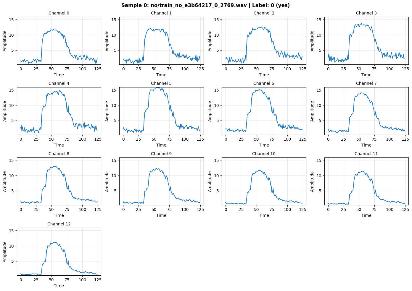
def inspect_batch(batch_data, batch_labels, batch_filenames, idx=0):
    """
    Visualize the filter outputs for a selected sample in a batch.

    Args:
        batch_data: Input tensor [B, T, C] - the filter outputs
        batch_labels: Labels tensor [B]
        batch_filenames: List of filenames
        idx: Index within the batch to display (0 to B-1)
    """
    B, T, C = batch_data.shape

    if idx < 0 or idx >= B:
        print(f"Error: idx must be between 0 and {B-1}")
        return

    sample = batch_data[idx].numpy()  # [T, C]
    label = batch_labels[idx].item()
    filename = batch_filenames[idx] if batch_filenames else "N/A"
    label_name = WORD_2 if label == 1 else WORD_1

    print(f"=== Sample {idx}/{B-1} ===")
    print(f"Filename: {filename}")
    print(f"Label: {label} ({label_name})")
    print(f"Shape: {sample.shape} (timesteps={T}, channels={C})")
    print(f"\nChannel statistics:")
    print(f"{'Ch':<4} {'Min':<8} {'Max':<8} {'Mean':<8} {'Sum':<10}")
    print("-" * 42)
    for ch in range(C):
        ch_data = sample[:, ch]
        print(f"{ch:<4} {ch_data.min():<8.4f} {ch_data.max():<8.4f} {ch_data.mean():<8.4f} {ch_data.sum():<10.2f}")

    print(f"\nTotal signal energy: {sample.sum():.2f}")

    # Plot channels
    n_rows = (C + 3) // 4
    fig, axes = plt.subplots(n_rows, 4, figsize=(14, 2.5 * n_rows))
    axes = axes.flatten()

    for ch in range(C):
        ax = axes[ch]
        ax.plot(sample[:, ch], linewidth=1.5)
        ax.set_title(f"Channel {ch}", fontsize=10)
        ax.set_xlabel("Time")
        ax.set_ylabel("Amplitude")
        ax.grid(True, alpha=0.3)
        ax.set_ylim(sample.min() - 0.1, sample.max() + 0.1)

    # Hide extra subplots
    for i in range(C, len(axes)):
        axes[i].axis('off')

    fig.suptitle(f"Sample {idx}: {filename} | Label: {label} ({label_name})", fontsize=12, fontweight='bold')
    plt.tight_layout()
    plt.show()

    return sample

# Inspect first sample
_ = inspect_batch(x, y, fn, idx=0)

=== Sample 0/15 ===
Filename: no/train_no_e3b64217_0_2769.wav
Label: 0 (yes)
Shape: (125, 13) (timesteps=125, channels=13)

Channel statistics:
Ch   Min      Max      Mean     Sum       
------------------------------------------
0    0.6270   11.8154  4.9269   615.86    
1    0.5980   12.2469  5.3056   663.19    
2    0.6940   12.5848  5.6825   710.31    
3    1.0199   13.7716  6.0802   760.02    
4    0.9684   14.7949  6.2851   785.63    
5    0.9089   15.7776  6.3329   791.61    
6    1.1963   15.1036  5.9569   744.61    
7    0.9939   14.0545  5.3820   672.75    
8    0.8402   13.0538  4.8206   602.58    
9    0.7941   12.3049  4.4441   555.52    
10   0.6298   11.6839  4.0651   508.14    
11   0.5092   11.2975  3.8292   478.65    
12   0.4650   11.2208  3.7257   465.71

Total signal energy: 8354.59

png

(Optional) Save/Load dataloader

torch.save(train_loader, "train_commands.pt")
torch.save(val_loader, "val_commands.pt")

train_loader = torch.load("train_commands.pt", weights_only=False)
val_loader = torch.load("val_commands.pt", weights_only=False)

3. LIFLayer vs HWLayer: Key Differences

Tutorial 1 (LIFLayer) vs Tutorial 2 (HWLayer)

Feature	LIFLayer (Tutorial 1)	HWLayer (Tutorial 2)
Purpose	Software-optimized LIF neurons	Hardware-deployable neurons
Weight Precision	Full 32-bit floating point	Quantized (configurable bits)
Hardware Deployment	Simulation only	Direct chip deployment
Neuron Model	Standard LIF dynamics	Hardware-constrained LIF
Mismatch Modeling	Not included	Device variability simulation
Power Estimation	Not available	Built-in consumption metrics
Use Case	Research, prototyping	Production deployment

When to use each:

Use LIFLayer (Tutorial 1) for:
- Fast prototyping and experimentation
- Complex network architectures
- Research and algorithm development
Use HWLayer (Tutorial 2) for:
- Models targeting hardware deployment
- Power-constrained applications
- Realistic performance estimation
- Production neuromorphic systems

Hardware Constraints and Custom Losses

When deploying models to the Neuronova chip, several hardware constraints must be respected during training.

1. Frontend Connection Constraint (Diagonal Connectivity)

The hardware frontend consists of analog filters that are directly hardwired to input neurons in a 1-to-1 mapping:

Each filter connects to exactly one neuron (diagonal connectivity)
The weight "matrix" is actually just a 1D vector (N weights, not N×N)
All weights should be POSITIVE because input should excite neurons, not inhibit them

Filter 0 ──[w₀]──► Neuron 0
Filter 1 ──[w₁]──► Neuron 1
   ...              ...
Filter N ──[wₙ]──► Neuron N

The Frontend class automatically enforces this by storing only diagonal weights as a 1D parameter vector and using element-wise multiplication instead of matrix multiplication.

2. Weight Magnitude Constraint

Synaptic weights are stored in analog memories with a limited dynamic range. Weights exceeding this range cannot be accurately programmed.

Solution: weight_magnitude_loss(model, limit=0.9) penalizes weights exceeding the limit:

\[\mathcal{L}_{wm} = \frac{1}{N}\sum_{i} \text{ReLU}(|w_i| - \text{limit})^2\]

3. Sign Alignment Constraint (Topology Loss)

Due to hardware architecture, groups of 5 contiguous synapses must share the same sign.

Solution: topology_loss(model, lam) encourages sign alignment within groups:

Group 0: weights[0:5]   → should all be positive OR all negative
Group 1: weights[5:10]  → should all be positive OR all negative
...

Note: This constraint applies to core layers (HWSynapse), not the frontend.

Combined Loss Function

loss = loss_task + topology_loss(model, lam=0.5) + weight_magnitude_loss(model, limit=0.9)

4. Hardware-Ready SNN Model

We build a 3-layer spiking network using Frontend, HWSynapse, and HWLayer:

Architecture:

Input [B, T, C] → Frontend (diagonal) → HWLayer [B, T, C]
                                              ↓
                    HWSynapse (dense) → HWLayer [B, T, 64] (hidden)
                                              ↓
                    HWSynapse (dense) → HWLayer [B, T, 2] (output)

Classification method: Spike count comparison (no separate readout layer)

Training Tip: Learning Rate for Frontend

Since the Frontend has only N weights (one per channel) compared to dense layers with N×M weights, the frontend weights:

Have fewer parameters to distribute gradient across
Receive stronger per-weight gradients
Can become unstable with high learning rates

Recommendation: Use a smaller learning rate for the Frontend (e.g., 10-100x smaller than core layers):

optimizer = torch.optim.Adam([
    {'params': frontend.parameters(), 'lr': 1e-5},  # Smaller LR for frontend
    {'params': core_net.parameters(), 'lr': 1e-3},  # Normal LR for core
])

This prevents the frontend weights from changing too rapidly and makes training more stable.

class FrontendNet(nn.Module):
    """
    Frontend layer with DIAGONAL connectivity (1-to-1 filter-to-neuron mapping).

    The Neuronova chip's frontend has analog filters hardwired to input neurons:
    - Each input channel i connects ONLY to neuron i
    - Weight matrix is diagonal → stored as 1D vector [N] instead of [N, N]
    - Forward pass: output = input * weights (element-wise, not matmul)

    This saves parameters: N weights instead of N² for an N-channel input.
    """
    def __init__(self, dt=8e-3, n_channels=16):
        super().__init__()

        # Frontend synapse: diagonal connectivity (N weights for N channels)
        # init: positive values since input should excite neurons
        self.frontend_syn = Frontend(
            nb_inputs=n_channels,
            init=lambda w: nn.init.normal_(w, 0.1, 0.01),  # Small positive weights
        )

        # LIF neurons for the frontend layer
        self.hw1 = HWLayer(
            n_neurons=n_channels, 
            taus=10e-3,  # 10ms membrane time constant
            dt=dt, 
            spike_grad=fast_sigmoid(slope=25.0)
        )

    def forward(self, x):  # x: [B, T, N]
        B, T, _ = x.shape

        mem_trace = []
        spk_trace = []
        cur_trace = []

        # Reset neuron states and build conductance matrices
        prepare_net(self)

        for t in range(T):
            # Diagonal synapse: element-wise multiplication (not matmul)
            cur1 = self.frontend_syn(x[:, t, :])
            cur_trace.append(cur1)

            # LIF neuron dynamics
            spk1, mem1 = self.hw1(cur1)
            mem_trace.append(mem1)
            spk_trace.append(spk1)

        mem_trace = torch.stack(mem_trace, dim=1)  # [B, T, N]
        spk_trace = torch.stack(spk_trace, dim=1)  # [B, T, N]
        self.cur_trace = torch.stack(cur_trace, dim=1)  # [B, T, N]

        return spk_trace


class HWSNN(nn.Module):
    """
    Hardware-ready SNN core with hidden layer using DENSE connectivity.

    Architecture:
        Frontend spikes [B, T, C] 
            → Hidden layer (HWSynapse + HWLayer) [B, T, hidden_size]
            → Output layer (HWSynapse + HWLayer) [B, T, num_classes]

    Unlike Frontend, HWSynapse uses full matrix multiplication (dense connectivity)
    where each input neuron connects to ALL output neurons.
    """
    def __init__(self, n_channels, num_classes=2, hidden_size=32, dt=8e-3):
        super().__init__()
        self.hidden_size = hidden_size
        self.num_classes = num_classes
        self.dt = dt

        taus = 64e-3  # 64ms membrane time constant

        # Hidden layer: full connectivity (n_channels × hidden_size weights)
        self.syn_hidden = HWSynapse(
            n_channels, hidden_size, 
            init=lambda w: nn.init.normal_(w, 0.1, 0.3)
        )
        self.hw_hidden = HWLayer(
            n_neurons=hidden_size, 
            taus=taus, 
            dt=dt, 
            spike_grad=fast_sigmoid(slope=25.0)
        )

        # Output layer: full connectivity (hidden_size × num_classes weights)
        self.syn_out = HWSynapse(
            hidden_size, num_classes, 
            init=lambda w: nn.init.normal_(w, 0.1, 0.3),
        )
        self.hw_out = HWLayer(
            n_neurons=num_classes, 
            taus=taus, 
            dt=dt, 
            spike_grad=fast_sigmoid(slope=25.0)
        )

    def forward(self, x):
        """
        Forward pass: process spikes through hidden and output layers.

        Args:
            x: Input tensor [B, T, N] (frontend spikes)

        Returns:
            spk_trace: Output spikes [B, T, num_classes]
        """
        B, T, _ = x.shape

        spk_hidden_trace = []
        spk_out_trace = []

        # Reset neuron states and build conductance matrices
        prepare_net(self)

        for t in range(T):
            # Hidden layer: dense synaptic connection + LIF dynamics
            cur_hidden = self.syn_hidden(x[:, t, :])
            spk_hidden, mem_hidden = self.hw_hidden(cur_hidden)
            spk_hidden_trace.append(spk_hidden)

            # Output layer: dense synaptic connection + LIF dynamics
            cur_out = self.syn_out(spk_hidden)
            spk_out, mem_out = self.hw_out(cur_out)
            spk_out_trace.append(spk_out)

        self.spk_hidden_trace = torch.stack(spk_hidden_trace, dim=1)
        self.spk_out_trace = torch.stack(spk_out_trace, dim=1)

        return self.spk_out_trace


# ============================================
# MODEL INSTANTIATION
# ============================================
torch.manual_seed(42)

HIDDEN_SIZE = 64

frontend = FrontendNet(n_channels=N_CHANNELS).to(device)
core_net = HWSNN(n_channels=N_CHANNELS, hidden_size=HIDDEN_SIZE).to(device)
model = nn.Sequential(frontend, core_net)

criterion = nn.CrossEntropyLoss()

# IMPORTANT: Use different learning rates for frontend vs core
# Frontend has only N weights (diagonal) vs many more in core layers
# Smaller LR prevents frontend weights from changing too rapidly
optimizer = torch.optim.Adam([
    {'params': frontend.parameters(), 'lr': 1e-5},  # 100x smaller for frontend stability
    {'params': core_net.parameters(), 'lr': 1e-3},  # Normal LR for dense layers
])

print("=== Hardware-Ready Model ===")
print(model)
print(f"\nTotal parameters: {sum(p.numel() for p in model.parameters()):,}")

print(f"\n=== Frontend Synapse (Diagonal: 1-to-1 mapping) ===")
print(f"Weight shape: {frontend.frontend_syn.weight.shape} (1D vector, NOT matrix)")
print(f"Parameters: {frontend.frontend_syn.weight.numel()} (one per channel)")

print(f"\n=== Hidden Layer (Dense: all-to-all) ===")
print(f"Synapse shape: {core_net.syn_hidden.weight.shape}")
print(f"Parameters: {core_net.syn_hidden.weight.numel()}")

print(f"\n=== Output Layer (Dense: all-to-all) ===")
print(f"Synapse shape: {core_net.syn_out.weight.shape}")
print(f"Parameters: {core_net.syn_out.weight.numel()}")

=== Hardware-Ready Model ===
Sequential(
  (0): FrontendNet(
    (frontend_syn): Frontend()
    (hw1): HWLayer(
      (spike_grad): FastSigmoid(slope=25.0)
    )
  )
  (1): HWSNN(
    (syn_hidden): HWSynapse()
    (hw_hidden): HWLayer(
      (spike_grad): FastSigmoid(slope=25.0)
    )
    (syn_out): HWSynapse()
    (hw_out): HWLayer(
      (spike_grad): FastSigmoid(slope=25.0)
    )
  )
)

Total parameters: 973

=== Frontend Synapse (Diagonal: 1-to-1 mapping) ===
Weight shape: torch.Size([13]) (1D vector, NOT matrix)
Parameters: 13 (one per channel)

=== Hidden Layer (Dense: all-to-all) ===
Synapse shape: torch.Size([13, 64])
Parameters: 832

=== Output Layer (Dense: all-to-all) ===
Synapse shape: torch.Size([64, 2])
Parameters: 128


/tmp/ipykernel_3077550/2921699216.py:17: UserWarning: Frontend on chip uses 16 filters. Using a different amount of neurons 13 is allowed but not respecting the chip constraints.
  self.frontend_syn = Frontend(

# ============================================
# CHECK INITIAL FIRING RATES (before training)
# ============================================
# This is critical to verify the initialization isn't too high (saturated)
# or too low (dead neurons). Target: 10-50% firing rate for healthy learning.

def check_firing_rates(model, frontend, core_net, loader, n_batches=3):
    """
    Check firing rates for frontend and core layers.

    Healthy ranges:
    - Frontend: 10-60% (should respond to input signal)
    - Core: 10-50% (should have room to differentiate classes)

    Warning signs:
    - >90%: Neurons saturated (weights too high)
    - <5%: Neurons barely firing (weights too low)
    """
    model.eval()

    frontend_frs = []
    core_frs_n0 = []
    core_frs_n1 = []

    with torch.no_grad():
        for i, (specs, labels, fn) in enumerate(loader):
            if i >= n_batches:
                break

            specs = specs.to(device)

            # Get frontend spikes
            frontend_spk = frontend(specs)

            # Get core spikes (full model output)
            core_spk = model(specs)

            # Per-channel frontend firing rates
            frontend_fr_per_ch = frontend_spk.mean(dim=(0, 1))
            frontend_frs.append(frontend_fr_per_ch)

            # Per-neuron core firing rates
            core_frs_n0.append(core_spk[:, :, 0].mean().item())
            core_frs_n1.append(core_spk[:, :, 1].mean().item())

    # Average across batches
    frontend_fr_avg = torch.stack(frontend_frs).mean(dim=0)
    core_fr_n0 = np.mean(core_frs_n0)
    core_fr_n1 = np.mean(core_frs_n1)

    print("=" * 60)
    print("INITIAL FIRING RATES CHECK (before training)")
    print("=" * 60)

    print(f"\n{'Layer':<20} {'Firing Rate':<15} {'Status'}")
    print("-" * 50)

    # Frontend per-channel
    print(f"\n=== Frontend Layer ({N_CHANNELS} channels) ===")
    for ch in range(N_CHANNELS):
        fr = frontend_fr_avg[ch].item()
        if fr > 0.9:
            status = "WARNING: Saturated!"
        elif fr < 0.05:
            status = "WARNING: Too low!"
        elif fr < 0.1:
            status = "Low"
        elif fr > 0.7:
            status = "High"
        else:
            status = "OK"
        print(f"  Channel {ch:<3}        {fr*100:>6.1f}%         {status}")

    frontend_mean = frontend_fr_avg.mean().item()
    print(f"\n  Frontend MEAN:     {frontend_mean*100:>6.1f}%")

    # Core layer
    print(f"\n=== Core Layer (2 output neurons) ===")
    for i, fr in enumerate([core_fr_n0, core_fr_n1]):
        if fr > 0.9:
            status = "WARNING: Saturated!"
        elif fr < 0.05:
            status = "WARNING: Too low!"
        elif fr < 0.1:
            status = "Low"
        elif fr > 0.7:
            status = "High"
        else:
            status = "OK"
        word = WORD_1 if i == 0 else WORD_2
        print(f"  Neuron {i} ({word}): {fr*100:>6.1f}%         {status}")

    print("\n" + "-" * 50)
    print("Target: 10-50% for healthy gradient flow")
    print("=" * 60)

    return frontend_fr_avg, core_fr_n0, core_fr_n1

# Run the check
frontend_fr, core_n0_fr, core_n1_fr = check_firing_rates(model, frontend, core_net, train_loader)

============================================================
INITIAL FIRING RATES CHECK (before training)
============================================================

Layer                Firing Rate     Status
--------------------------------------------------

=== Frontend Layer (13 channels) ===
  Channel 0            37.5%         OK
  Channel 1            38.1%         OK
  Channel 2            38.5%         OK
  Channel 3            38.4%         OK
  Channel 4            32.5%         OK
  Channel 5            36.6%         OK
  Channel 6            43.9%         OK
  Channel 7            32.5%         OK
  Channel 8            36.1%         OK
  Channel 9            34.2%         OK
  Channel 10           34.4%         OK
  Channel 11           34.6%         OK
  Channel 12           35.8%         OK

  Frontend MEAN:       36.4%

=== Core Layer (2 output neurons) ===
  Neuron 0 (yes):   55.2%         OK
  Neuron 1 (no):   18.4%         OK

--------------------------------------------------
Target: 10-50% for healthy gradient flow
============================================================

5. Training the Hardware Model

Training proceeds identically to standard PyTorch models. The hardware constraints are automatically handled by HWLayer.

from nwavesdk.loss import firing_rate_target_mse_loss
from nwavesdk.metrics import accuracy

def evaluate(model, loader):
    """Evaluate model accuracy on a dataloader."""
    model.eval()
    correct = 0
    total = 0

    with torch.no_grad():
        for specs, labels, fn in loader:
            specs = specs.to(device)
            labels = labels.to(device)

            spike_traces = model(specs)
            correct += accuracy(spike_traces, labels)
            total += 1

    return correct / max(total, 1)



# ============================================
# TRAINING HYPERPARAMETERS
# ============================================
HP = {
    'epochs': 40,
    'lam_topology': 0.05,     # Topology constraint weight
    'lam_fr': 10,             # Firing rate regularization
    'target_fr': 0.15,        # Target firing rate
    'lr_frontend': 1e-5,      # Learning rate for frontend (smaller for stability)
    'lr_core': 1e-3,          # Learning rate for core layers
}

# Reinitialize optimizer with separate learning rates
optimizer = torch.optim.Adam([
    {'params': frontend.parameters(), 'lr': HP['lr_frontend']},
    {'params': core_net.parameters(), 'lr': HP['lr_core']},
])

# ============================================
# TRAINING HISTORY
# ============================================
history = {
    'train_loss': [], 'loss_main': [], 'loss_topo': [], 'loss_fr': [],
    'train_acc': [], 'val_acc': [], 'fr_n0': [], 'fr_n1': [],
}

best_acc = 0.0
best_state = None

print(f"\n=== Training Hardware Model ({WORD_1} vs {WORD_2}) ===")
print(f"Frontend LR: {HP['lr_frontend']} | Core LR: {HP['lr_core']}")
print(f"Topology λ: {HP['lam_topology']} | FR λ: {HP['lam_fr']} | Target FR: {HP['target_fr']}\n")
print(f"{'Epoch':<6} | {'Loss':<7} | {'L_main':<7} | {'Train':<7} | {'Val':<7} | {'FR_n0':<6} | {'FR_n1':<6} | {'Best':<5}")
print("=" * 75)

for epoch in range(1, HP['epochs'] + 1):
    model.train()
    running_loss, running_main, running_topo, running_fr = 0.0, 0.0, 0.0, 0.0
    train_correct, train_total = 0, 0

    for specs, labels, fn in train_loader:
        specs, labels = specs.to(device), labels.to(device)

        optimizer.zero_grad()

        # Forward pass
        spike_counts = model(specs)
        logits = spike_counts.sum(dim=1)

        # Loss computation
        loss_main = criterion(logits, labels)
        loss_topo = topology_loss(core_net, lam=HP['lam_topology'])
        loss_mag  = weight_magnitude_loss(core_net)
        # we want both neurons to fire at 15%, the cleanest way to achieve is with the mse loss, but not on the layer directly (since would make the average firing rate of the layer regret to 15%), but directly on neurons axis
        loss_fr   = HP['lam_fr'] * firing_rate_target_mse_loss(spikes_list = [spike_counts[:, :, 0].unsqueeze(1),  spike_counts[:, :, 1].unsqueeze(1),], offsets = [HP['target_fr']] * 2, multipliers = [1] * 2)

        loss = loss_main + loss_fr + loss_topo + loss_mag
        loss.backward()

        torch.nn.utils.clip_grad_norm_(model.parameters(), max_norm=0.5)
        optimizer.step()


        preds = logits.argmax(dim=1)
        train_correct += (preds == labels).sum().item()
        train_total += labels.size(0)

        batch_size = labels.size(0)
        running_loss += loss.item() * batch_size
        running_main += loss_main.item() * batch_size
        running_fr += loss_fr.item() * batch_size

    # Epoch statistics
    n_samples = len(train_loader.dataset)
    epoch_loss = running_loss / n_samples
    epoch_main = running_main / n_samples
    epoch_fr = running_fr / n_samples
    train_acc = train_correct / train_total
    val_acc = evaluate(model, val_loader)

    # Get firing rates
    model.eval()
    with torch.no_grad():
        for specs, labels, fn in train_loader:
            out = model(specs.to(device))
            fr_n0 = out[:, :, 0].mean().item()
            fr_n1 = out[:, :, 1].mean().item()
            break

    # Store history
    history['train_loss'].append(epoch_loss)
    history['loss_main'].append(epoch_main)
    history['loss_topo'].append(0)
    history['loss_fr'].append(epoch_fr)
    history['train_acc'].append(train_acc)
    history['val_acc'].append(val_acc)
    history['fr_n0'].append(fr_n0)
    history['fr_n1'].append(fr_n1)

    # Track best model
    is_best = ""
    if val_acc > best_acc:
        best_acc = val_acc
        best_state = {k: v.clone() for k, v in model.state_dict().items()}
        is_best = "★"

    if epoch % 5 == 0 or epoch == 1 or is_best:
        print(f"{epoch:<6} | {epoch_loss:<7.4f} | {epoch_main:<7.4f} | {train_acc:<7.1%} | {val_acc:<7.1%} | {fr_n0:<6.3f} | {fr_n1:<6.3f} | {is_best}")



# Restore best model
if best_state is not None:
    model.load_state_dict(best_state)
    print(f"\nRestored best model with validation accuracy: {best_acc:.1%}")

print("=" * 75)
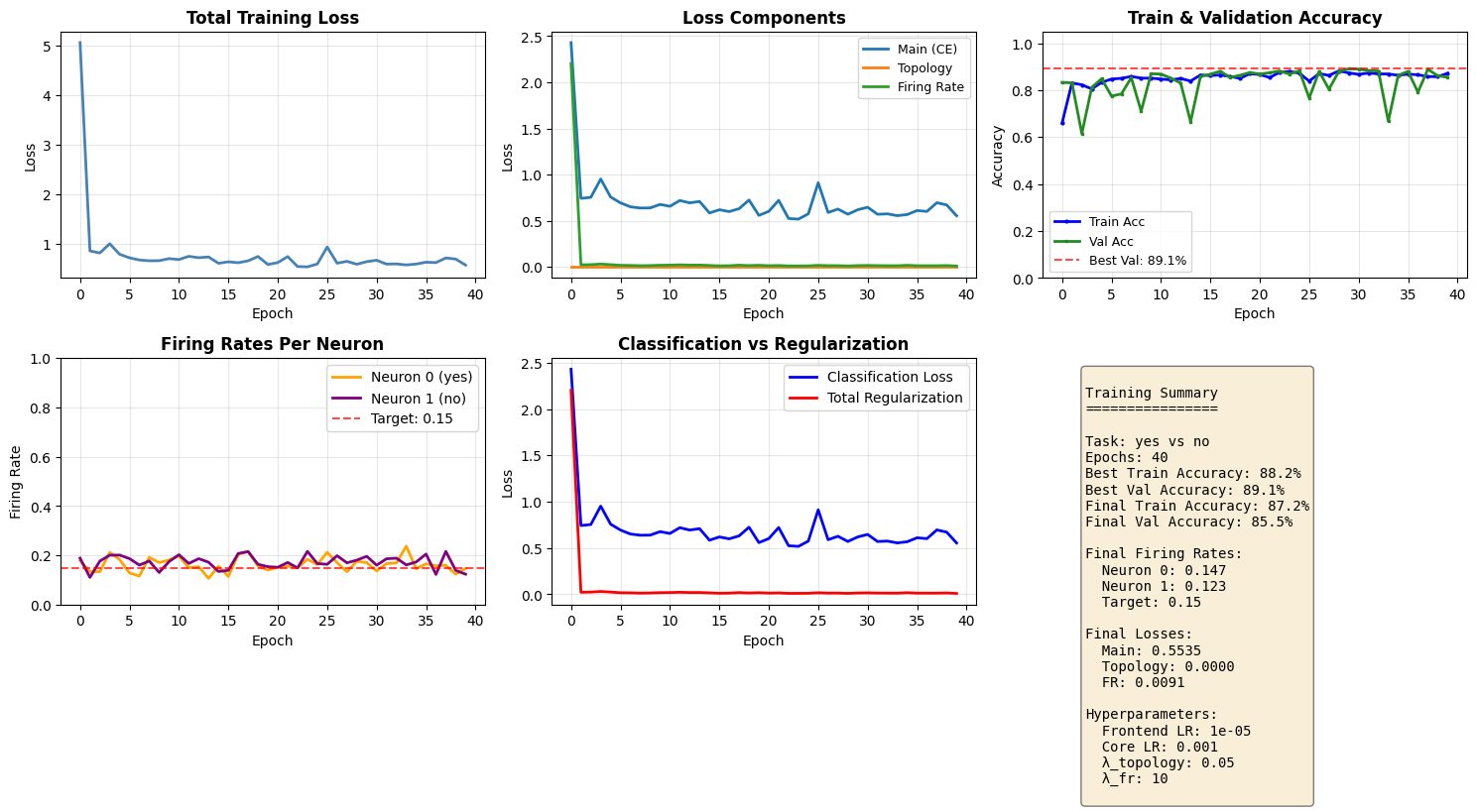
print(f"\nTraining completed! Best validation accuracy: {best_acc:.1%}")

=== Training Hardware Model (yes vs no) ===
Frontend LR: 1e-05 | Core LR: 0.001
Topology λ: 0.05 | FR λ: 10 | Target FR: 0.15

Epoch  | Loss    | L_main  | Train   | Val     | FR_n0  | FR_n1  | Best 
===========================================================================
1      | 5.0588  | 2.4294  | 66.0%   | 83.3%   | 0.178  | 0.189  | ★
5      | 0.7821  | 0.7569  | 83.3%   | 84.8%   | 0.183  | 0.201  | ★
8      | 0.6502  | 0.6376  | 85.8%   | 85.3%   | 0.192  | 0.177  | ★
10     | 0.6937  | 0.6761  | 85.1%   | 86.9%   | 0.181  | 0.175  | ★
15     | 0.5991  | 0.5837  | 86.4%   | 85.8%   | 0.155  | 0.134  | 
17     | 0.6111  | 0.5988  | 86.5%   | 88.1%   | 0.204  | 0.207  | ★
20     | 0.5751  | 0.5576  | 87.0%   | 87.5%   | 0.140  | 0.154  | 
23     | 0.5340  | 0.5240  | 87.5%   | 88.1%   | 0.149  | 0.149  | ★
25     | 0.5850  | 0.5741  | 87.2%   | 88.2%   | 0.162  | 0.167  | ★
30     | 0.6328  | 0.6190  | 87.4%   | 89.1%   | 0.170  | 0.196  | ★
35     | 0.5841  | 0.5669  | 86.3%   | 86.3%   | 0.146  | 0.173  | 
40     | 0.5626  | 0.5535  | 87.2%   | 85.5%   | 0.147  | 0.123  |

Restored best model with validation accuracy: 89.1%
===========================================================================

Training completed! Best validation accuracy: 89.1%

Training Convergence Plots

fig, axes = plt.subplots(2, 3, figsize=(15, 8))

# Plot 1: Total training loss
ax = axes[0, 0]
ax.plot(history['train_loss'], linewidth=2, color='steelblue')
ax.set_title('Total Training Loss', fontsize=12, fontweight='bold')
ax.set_xlabel('Epoch')
ax.set_ylabel('Loss')
ax.grid(True, alpha=0.3)

# Plot 2: Individual losses
ax = axes[0, 1]
ax.plot(history['loss_main'], label='Main (CE)', linewidth=2)
ax.plot(history['loss_topo'], label='Topology', linewidth=2)
ax.plot(history['loss_fr'], label='Firing Rate', linewidth=2)
ax.set_title('Loss Components', fontsize=12, fontweight='bold')
ax.set_xlabel('Epoch')
ax.set_ylabel('Loss')
ax.legend(fontsize=9)
ax.grid(True, alpha=0.3)

# Plot 3: Train & Validation accuracy
ax = axes[0, 2]
ax.plot(history['train_acc'], linewidth=2, color='blue', label='Train Acc', marker='o', markersize=2)
ax.plot(history['val_acc'], linewidth=2, color='forestgreen', label='Val Acc', marker='s', markersize=2)
ax.axhline(y=max(history['val_acc']), color='red', linestyle='--', alpha=0.7, label=f'Best Val: {max(history["val_acc"]):.1%}')
ax.set_title('Train & Validation Accuracy', fontsize=12, fontweight='bold')
ax.set_xlabel('Epoch')
ax.set_ylabel('Accuracy')
ax.set_ylim(0, 1.05)
ax.legend(fontsize=9)
ax.grid(True, alpha=0.3)

# Plot 4: Firing rates per neuron
ax = axes[1, 0]
ax.plot(history['fr_n0'], label=f'Neuron 0 ({WORD_1})', linewidth=2, color='orange')
ax.plot(history['fr_n1'], label=f'Neuron 1 ({WORD_2})', linewidth=2, color='purple')
ax.axhline(y=HP['target_fr'], color='red', linestyle='--', alpha=0.7, label=f'Target: {HP["target_fr"]}')
ax.set_title('Firing Rates Per Neuron', fontsize=12, fontweight='bold')
ax.set_xlabel('Epoch')
ax.set_ylabel('Firing Rate')
ax.set_ylim(0, 1.0)
ax.legend()
ax.grid(True, alpha=0.3)

# Plot 5: Main loss vs Regularization losses
ax = axes[1, 1]
total_reg = [t + f for t, f in zip(history['loss_topo'], history['loss_fr'])]
ax.plot(history['loss_main'], label='Classification Loss', linewidth=2, color='blue')
ax.plot(total_reg, label='Total Regularization', linewidth=2, color='red')
ax.set_title('Classification vs Regularization', fontsize=12, fontweight='bold')
ax.set_xlabel('Epoch')
ax.set_ylabel('Loss')
ax.legend()
ax.grid(True, alpha=0.3)

# Plot 6: Summary stats
ax = axes[1, 2]
ax.axis('off')
summary_text = f"""
Training Summary
================

Task: {WORD_1} vs {WORD_2}
Epochs: {len(history['train_loss'])}
Best Train Accuracy: {max(history['train_acc']):.1%}
Best Val Accuracy: {max(history['val_acc']):.1%}
Final Train Accuracy: {history['train_acc'][-1]:.1%}
Final Val Accuracy: {history['val_acc'][-1]:.1%}

Final Firing Rates:
  Neuron 0: {history['fr_n0'][-1]:.3f}
  Neuron 1: {history['fr_n1'][-1]:.3f}
  Target: {HP['target_fr']}

Final Losses:
  Main: {history['loss_main'][-1]:.4f}
  Topology: {history['loss_topo'][-1]:.4f}
  FR: {history['loss_fr'][-1]:.4f}

Hyperparameters:
  Frontend LR: {HP['lr_frontend']}
  Core LR: {HP['lr_core']}
  λ_topology: {HP['lam_topology']}
  λ_fr: {HP['lam_fr']}
"""
ax.text(0.1, 0.95, summary_text, transform=ax.transAxes, fontsize=10,
        verticalalignment='top', fontfamily='monospace',
        bbox=dict(boxstyle='round', facecolor='wheat', alpha=0.5))

plt.tight_layout()
plt.show()

png

6. Saving and Loading Models

NWAVE models are fully compatible with PyTorch's save/load mechanism. You can save and load models just like any standard PyTorch model.

Two methods:

Save full model (architecture + weights)
Save state dict (weights only - recommended)

# Method 1: Save state dict (recommended)
model_filename = f'hwsnn_{WORD_1}_{WORD_2}.pth'
torch.save(model.state_dict(), model_filename)
print(f"Model weights saved to '{model_filename}'")

# Method 2: Save full model (optional)
model_full_filename = f'hwsnn_{WORD_1}_{WORD_2}_full.pth'
torch.save(model, model_full_filename)
print(f"Full model saved to '{model_full_filename}'")

Model weights saved to 'hwsnn_yes_no.pth'
Full model saved to 'hwsnn_yes_no_full.pth'

Load Model and Verify

# To load the model, recreate the architecture with THE SAME PARAMETERS
# IMPORTANT: hidden_size and n_channels must match what was used during training!

loaded_frontend = FrontendNet(n_channels=N_CHANNELS).to(device)
loaded_core = HWSNN(n_channels=N_CHANNELS, hidden_size=HIDDEN_SIZE).to(device)
loaded_model = nn.Sequential(loaded_frontend, loaded_core)

# Load the saved weights
loaded_model.load_state_dict(torch.load(model_filename))
loaded_model.eval()

print("Model loaded successfully!\n")

# Verify the loaded model works correctly
loaded_acc = evaluate(loaded_model, val_loader)
original_acc = evaluate(model, val_loader)

print(f"Original model accuracy: {original_acc:.1%}")
print(f"Loaded model accuracy:   {loaded_acc:.1%}")
print(f"\nMatch: {abs(loaded_acc - original_acc) < 0.01}" + (" ✓" if abs(loaded_acc - original_acc) < 0.01 else " - Mismatch!"))

Model loaded successfully!



/tmp/ipykernel_3077550/2921699216.py:17: UserWarning: Frontend on chip uses 16 filters. Using a different amount of neurons 13 is allowed but not respecting the chip constraints.
  self.frontend_syn = Frontend(


Original model accuracy: 89.1%
Loaded model accuracy:   89.1%

Match: True ✓

7. Hardware Power Consumption Analysis

One of the key advantages of HWLayer is the ability to estimate power consumption for hardware deployment using the built-in get_chip_consumption() function.

Power Model

The Neuronova chip power consumption consists of two components:

Static Power:
- Always consumed when chip is used
- Dominates in low-activity scenarios
Dynamic Power: Energy per spike
- Only consumed when neurons fire
- Proportional to spike rate

Total Power = (Static Power × # Neurons) + (Dynamic Power from all spikes)

This event-driven power model is why SNNs are extremely energy-efficient compared to traditional ANNs.

# Run inference and collect spike data for power analysis
model.eval()
all_spk_hidden = []
all_spk_output = []

with torch.no_grad():
    for specs, labels, fn in val_loader:
        specs = specs.to(device)
        spk_frontend = frontend(specs)
        spk_output = core_net(spk_frontend)
        all_spk_hidden.append(core_net.spk_hidden_trace)
        all_spk_output.append(spk_output)

all_spk_hidden = torch.cat(all_spk_hidden, dim=0)
all_spk_output = torch.cat(all_spk_output, dim=0)

# Create flat model with core HW layers
# Note: Frontend excluded as it has 1D diagonal weights
hw_model = nn.Sequential(
    core_net.syn_hidden,     # HWSynapse
    core_net.hw_hidden,      # HWLayer
    core_net.syn_out,        # HWSynapse
    core_net.hw_out,         # HWLayer
)

# Spike traces for each synapse layer
spks = [all_spk_hidden, all_spk_output]

# Compute power consumption
total_power = get_chip_consumption(hw_model, spks, dt=core_net.dt)

# Display results
n_timesteps = all_spk_hidden.shape[1]
energy_per_inference = total_power * n_timesteps * core_net.dt

print("="*50)
print(f"HARDWARE POWER CONSUMPTION ({WORD_1} vs {WORD_2})")
print("="*50)
print(f"Total power:           {total_power*1e6:.3f} uW")
print(f"Energy per inference:  {energy_per_inference*1e9:.3f} nJ")
print(f"\nSpike rates:")
print(f"  Hidden layer: {all_spk_hidden.mean().item()*100:.1f}%")
print(f"  Output layer: {all_spk_output.mean().item()*100:.1f}%")

==================================================
HARDWARE POWER CONSUMPTION (yes vs no)
==================================================
Total power:           0.016 uW
Energy per inference:  15.969 nJ

Spike rates:
  Hidden layer: 49.4%
  Output layer: 17.7%

8. Bonus: plotting neuron activity

We first grab the one batch of the inference

from nwavesdk.utils import plot_spike_raster
for specs, labels, fn in val_loader:
    specs = specs.to(device)
    spk_frontend = frontend(specs)
    spk_output = core_net(spk_frontend)
    target = labels
    break

Assume we want to plot the activity of the net given the second element of the batch.

sample_idx = 1

plot_spike_raster(
    spks,
    sample_idx = sample_idx,
    savepath=None,
)

png

Inspecting the classification layer and its prediciton we may get some insight about the prediction

plot_spike_raster(
    [spk_output],
    sample_idx = sample_idx,
    savepath=None,
)
print(target[sample_idx])

print(f"Class 0 logit: {spk_output[sample_idx, :, 0].sum()} | Class 1 logit: {spk_output[sample_idx, :, 1].sum()}")

png

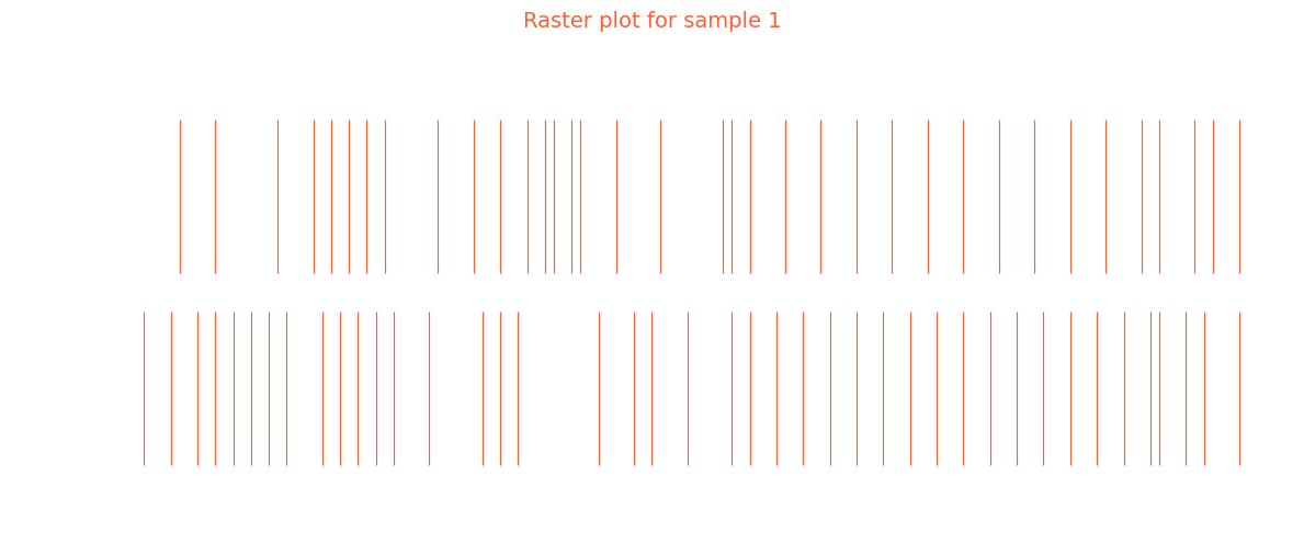
tensor(0)
Class 0 logit: 42.0 | Class 1 logit: 36.0

9. Summary

What We Learned

1. Hardware-Ready Models with HWLayer and Frontend

Frontend: Diagonal connectivity (1-to-1 filter-to-neuron mapping) - only N trainable weights
HWSynapse: Dense connectivity (all-to-all) - N×M trainable weights
HWLayer: Hardware-accurate spiking neurons with membrane dynamics

2. Key NWAVE Functions

Function	Purpose
`Frontend(nb_inputs, ...)`	Diagonal synaptic layer for analog frontend emulation
`HWSynapse(nb_in, nb_out, ...)`	Dense synaptic connections between neuron layers
`HWLayer(n_neurons, taus, dt, ...)`	Hardware spiking neurons with configurable dynamics
`prepare_net(model)`	Reset states and build conductance matrices before forward pass
`topology_loss(model, lam)`	Regularize for sign alignment in groups of 5 synapses
`weight_magnitude_loss(model, limit)`	Penalize weights exceeding hardware dynamic range
`fast_sigmoid(slope)`	Surrogate gradient for backpropagation through spikes

3. Training Tips

Use smaller learning rate for Frontend (10-100x smaller than core) since it has fewer weights
Apply topology_loss and weight_magnitude_loss for hardware compliance
Monitor firing rates to ensure neurons are in a healthy range (10-50%)

4. PyTorch Compatibility

Standard torch.save() and torch.load() work seamlessly
Models can be saved, loaded, and deployed like any PyTorch model

Key Takeaways

Frontend has diagonal connectivity: N weights for N channels (not N×N)
HWSynapse has dense connectivity: full matrix multiplication
Use separate learning rates: smaller for Frontend, larger for core layers
Hardware constraint losses ensure models are deployable to Neuronova chips

Next Steps

Tutorial 3: Explore non-idealities (mismatch, quantization effects)
Experiment with different network architectures
Try other word pairs from the Speech Commands dataset
Optimize for lower power consumption
Deploy to Neuronova hardware for real-world inference