NWAVE Tutorial 7: Recurrent Pattern Generation on H1v2 Hardware Model
Feedforward networks classify by accumulating spikes over time, but they cannot generate structured temporal outputs — each timestep's output depends only on the current input. Recurrent networks feed their own spike output back as input, allowing the network to maintain state and produce time-varying patterns independently of the external drive.
This tutorial trains an H1v2 recurrent network to reproduce a target spike-rate pattern:
- RC (recurrent) topology on H1v2 — first use of
layer_topology="RC" - H1v2's lower synaptic gain requires more FF input channels than H1v1
fluct_initwithalpha<1to split the variance budget between feedforward and recurrent weights (alpha=1.0tunes only feedforward connections)- Pair with
chip-constraintsandinitializations/fluct_initpages on the official documentation
1. Setup and Imports
import matplotlib.pyplot as plt
import numpy as np
import torch
import torch.nn as nn
from torch.utils.data import DataLoader, TensorDataset

from nwavesdk.layers import H1v2Synapse, H1v2Layer, prepare_net
from nwavesdk.init.fluct_init import fluct_init
from nwavesdk.loss import weight_magnitude_loss
from nwavesdk.surrogate import fast_sigmoid

device = torch.device("cuda" if torch.cuda.is_available() else "cpu")
device_flag = "gpu" if device.type == "cuda" else "cpu"

torch.manual_seed(42)
np.random.seed(42)

print(f"Device: {device}")
nwavesdk version: 1.0.0a0+rocm
Device: cuda
2. Target pattern generation
def generate_temporal_targets(n_steps, n_neurons, pattern_type="sine"):
    t = torch.linspace(0, 4 * np.pi, n_steps)
    targets = torch.zeros(n_steps, n_neurons)
    if pattern_type == "sine":
        for i in range(n_neurons):
            phase = (2 * np.pi * i) / n_neurons
            targets[:, i] = 0.5 + 0.4 * torch.sin(t + phase)
    return targets


batch_size = 16
n_steps = 100
n_neurons = 8
n_inputs = 8      # H1v2 usually needs more FF inputs — see Section 3
dt = 1e-3
taus = 25e-3
surrogate_slope = 25.0
learning_rate = 5e-4
n_epochs = 5000
spike_prob = 0.4
n_samples = 128

target_pattern = generate_temporal_targets(n_steps, n_neurons, "sine").to(device)
x_train = (torch.rand(n_samples, n_steps, n_inputs) < spike_prob).float().to(device)
train_dl = DataLoader(TensorDataset(x_train), batch_size=batch_size, shuffle=True)

print(f"Input:  {x_train.shape}")
print(f"Target: {target_pattern.shape}")
Input:  torch.Size([128, 100, 8])
Target: torch.Size([100, 8])
3. Model definition: recurrent H1v2 network
RC topology. Setting layer_topology="RC" adds a learned recurrent weight matrix within the same layer. Each timestep, the layer receives both external input and its own previous spike output — allowing the network to maintain temporal state across the sequence.
H1v2 input width. H1v2 uses a linear synapse model with much lower synaptic gain per weight than H1v1. With a single input channel, the mean weight required to drive the membrane to threshold would exceed the hardware limit [-1.66, 1.66]. Using 8 input channels distributes the charge requirement across more weights, keeping each one within range. fluct_init will warn if initialized weights still fall outside the hardware range.
class H2PatternGenerator(nn.Module):
    """Recurrent H1v2 network for temporal pattern generation."""

    def __init__(self, n_neurons, taus, dt=1e-3):
        super().__init__()
        self.device_flag = device_flag
        self.synapse = H1v2Synapse(
            nb_inputs=n_inputs,
            nb_outputs=n_neurons,
            device=self.device_flag,
        )
        self.lif = H1v2Layer(
            n_neurons=n_neurons,
            taus=taus,
            dt=dt,
            layer_topology="RC",
            spike_grad=fast_sigmoid(slope=surrogate_slope),
            device=self.device_flag,
        )
        self.layer_pairs = [(self.synapse, self.lif)]

    def forward(self, x):
        prepare_net(self, collect_metrics=False)
        cur = self.synapse(x)
        if self.device_flag == "gpu":
            spk, mem = self.lif.forward_gpu(cur)
            return spk, mem

        spikes = []
        membranes = []
        for t in range(x.shape[1]):
            spk_t, mem_t = self.lif(cur[:, t, :])
            spikes.append(spk_t)
            membranes.append(mem_t)
        return torch.stack(spikes, dim=1), torch.stack(membranes, dim=1)


model = H2PatternGenerator(n_neurons=n_neurons, taus=taus, dt=dt).to(device)
print(model)

print("Applying fluct_init before training...")
fluct_init(
    model,
    train_dl,
    xi_target=2.0,
    alpha=0.85, # Variance budget between FF and RC connection, if 1 only FF connections are tuned
    n_batches=4,
    verbose=True,
)
H2PatternGenerator(
  (synapse): H1v2Synapse()
  (lif): H1v2Layer(
    (spike_grad): FastSigmoid(slope=25.0)
  )
)
Applying fluct_init before training...
[fluct_init] ξ=2.0  α=0.85  dt=1.0ms  (stacked, adaptive µ)  [H2]
  Input → ν_mean=401.5Hz  ν_var=401.5Hz  ratio=1.0x
  Layer 1 | ν_in=401.5Hz  µ_W=0.1772  σ_FF=0.2659  σ_RC=0.1342  µ_U=0.169
[fluct_init] done.
4. Training the recurrent network
Loss. MSE between the network's mean spike rate (averaged over the batch) and the target pattern. Mean spike rate is a continuous, differentiable proxy for spike probability and aligns with the smooth sine target — spike-timing losses are not needed here.
alpha=0.85 allocates 85 % of the variance budget to feedforward weights and 15 % to recurrent weights. The recurrent path carries fewer total inputs per neuron than the feedforward path, so it requires less initial drive to reach threshold.
optimizer = torch.optim.Adam(model.parameters(), lr=learning_rate)
model.train()
losses = []

for epoch in range(n_epochs):
    for (xb,) in train_dl:
        xb = xb.to(device)
        spikes, _ = model(xb)
        loss = (
            nn.functional.mse_loss(spikes.mean(dim=0), target_pattern)
            + weight_magnitude_loss(model, limit=1.66)
        )
        optimizer.zero_grad()
        loss.backward()
        nn.utils.clip_grad_norm_(model.parameters(), max_norm=1.0)
        optimizer.step()
    losses.append(loss.item())
    if (epoch + 1) % 200 == 0:
        print(f"Epoch {epoch + 1:4d}/{n_epochs} | Loss: {loss.item():.6f}")

print(f"Final loss: {losses[-1]:.6f}")
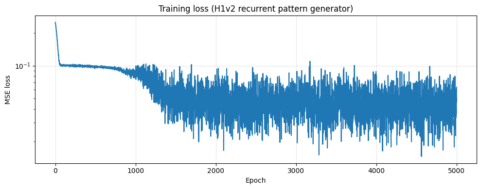
Epoch  200/5000 | Loss: 0.099999
Epoch  400/5000 | Loss: 0.097536
Epoch  600/5000 | Loss: 0.096736
Epoch  800/5000 | Loss: 0.093199
Epoch 1000/5000 | Loss: 0.088165
Epoch 1200/5000 | Loss: 0.075961
Epoch 1400/5000 | Loss: 0.061862
Epoch 1600/5000 | Loss: 0.045892
Epoch 1800/5000 | Loss: 0.054086
Epoch 2000/5000 | Loss: 0.072429
Epoch 2200/5000 | Loss: 0.059133
Epoch 2400/5000 | Loss: 0.061641
Epoch 2600/5000 | Loss: 0.049518
Epoch 2800/5000 | Loss: 0.023080
Epoch 3000/5000 | Loss: 0.050276
Epoch 3200/5000 | Loss: 0.048617
Epoch 3400/5000 | Loss: 0.044250
Epoch 3600/5000 | Loss: 0.038646
Epoch 3800/5000 | Loss: 0.035759
Epoch 4000/5000 | Loss: 0.082054
Epoch 4200/5000 | Loss: 0.052360
Epoch 4400/5000 | Loss: 0.041434
Epoch 4600/5000 | Loss: 0.031646
Epoch 4800/5000 | Loss: 0.052864
Epoch 5000/5000 | Loss: 0.063590
Final loss: 0.063590
5. Evaluation
plt.figure(figsize=(10, 4))
plt.plot(losses, linewidth=1.5)
plt.xlabel("Epoch")
plt.ylabel("MSE loss")
plt.title("Training loss (H1v2 recurrent pattern generator)")
plt.yscale("log")
plt.grid(True, alpha=0.3)
plt.tight_layout()
plt.show()

model.eval()
with torch.no_grad():
    x_test = (torch.rand(batch_size, n_steps, n_inputs, device=device) < spike_prob).float()
    y_test, _ = model(x_test)
    output = y_test.mean(dim=0).cpu().numpy()

target_np = target_pattern.cpu().numpy()
error = np.abs(output - target_np)

print(f"MSE: {np.mean((output - target_np) ** 2):.6f}")
print(f"MAE: {np.mean(error):.6f}")

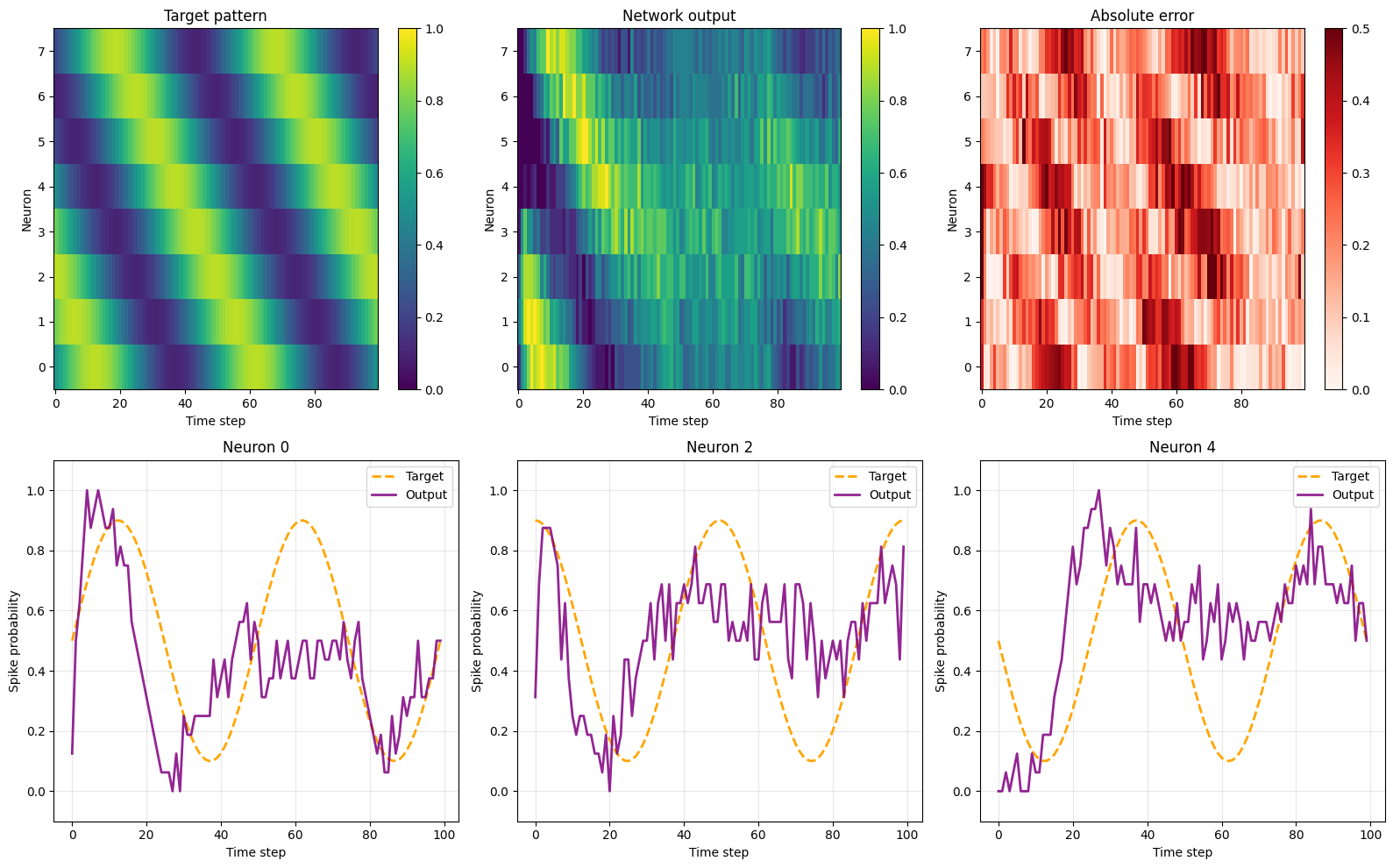
fig = plt.figure(figsize=(16, 10))
plt.subplot(2, 3, 1)
plt.imshow(target_np.T, aspect="auto", cmap="viridis", origin="lower", vmin=0, vmax=1)
plt.title("Target pattern")
plt.xlabel("Time step")
plt.ylabel("Neuron")
plt.colorbar()

plt.subplot(2, 3, 2)
plt.imshow(output.T, aspect="auto", cmap="viridis", origin="lower", vmin=0, vmax=1)
plt.title("Network output")
plt.xlabel("Time step")
plt.ylabel("Neuron")
plt.colorbar()

plt.subplot(2, 3, 3)
plt.imshow(error.T, aspect="auto", cmap="Reds", origin="lower", vmin=0, vmax=0.5)
plt.title("Absolute error")
plt.xlabel("Time step")
plt.ylabel("Neuron")
plt.colorbar()

for i, neuron_idx in enumerate([0, 2, 4]):
    plt.subplot(2, 3, 4 + i)
    plt.plot(target_np[:, neuron_idx], "--", linewidth=2, label="Target", color="orange")
    plt.plot(output[:, neuron_idx], linewidth=2, label="Output", color="purple", alpha=0.85)
    plt.xlabel("Time step")
    plt.ylabel("Spike probability")
    plt.title(f"Neuron {neuron_idx}")
    plt.grid(True, alpha=0.3)
    plt.ylim([-0.1, 1.1])
    plt.legend()

plt.tight_layout()
plt.show()
MSE: 0.062707
MAE: 0.209082
6. Analyzing learned weights
input_weights = model.synapse.weight.detach().cpu().numpy()
recurrent_weights = model.lif.recurrent_weights.detach().cpu().numpy()

fig, axes = plt.subplots(1, 2, figsize=(12, 4))
axes[0].imshow(input_weights, aspect="auto", cmap="RdBu_r",
               vmin=-np.abs(input_weights).max(), vmax=np.abs(input_weights).max())
axes[0].set_xlabel("Neuron index")
axes[0].set_ylabel("Input channel")
axes[0].set_title(f"Input weights (mean={input_weights.mean():.3f}, std={input_weights.std():.3f})")
plt.colorbar(axes[0].images[0], ax=axes[0], label="Weight")

im = axes[1].imshow(
    recurrent_weights,
    cmap="RdBu_r",
    vmin=-np.abs(recurrent_weights).max(),
    vmax=np.abs(recurrent_weights).max(),
)
axes[1].set_xlabel("Source neuron")
axes[1].set_ylabel("Target neuron")
axes[1].set_title(f"Recurrent weights (mean={recurrent_weights.mean():.3f})")
plt.colorbar(im, ax=axes[1], label="Weight")
plt.tight_layout()
plt.show()

print(f"Input weights     mean={input_weights.mean():.4f}, std={input_weights.std():.4f}")
print(f"Recurrent weights mean={recurrent_weights.mean():.4f}, std={recurrent_weights.std():.4f}")
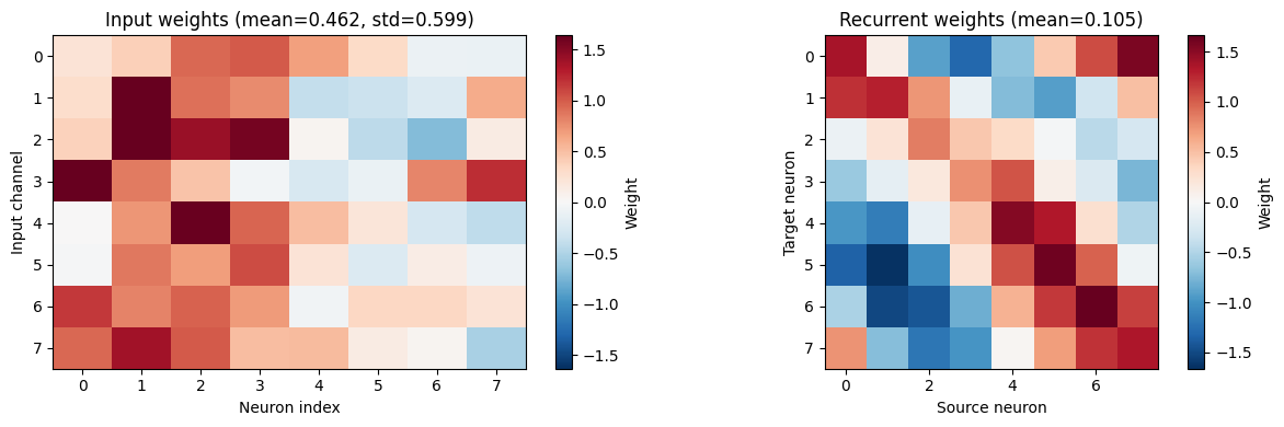
Input weights     mean=0.4620, std=0.5987
Recurrent weights mean=0.1047, std=0.9088
7. Summary
Recurrent H1v2 network with fluct_init, trained to generate a target spike-rate pattern:
| Value | Rationale | |
|---|---|---|
| RC topology | layer_topology="RC" |
Enables within-layer recurrence |
| FF inputs | 8 | H1v2's lower synaptic gain needs distributed charge |
| fluct_init ξ | 2.0 | Keeps init weights within [-1.66, 1.66] |
| fluct_init α | 0.85 | 85 % variance budget to FF, 15 % to recurrent |
| Training loss | MSE on mean spike rate | Differentiable proxy for spike probability |
| Weight constraint | weight_magnitude_loss(limit=1.66) |
Soft range enforcement during training |
For RC topology details and hardware deployment constraints see the official documentation (chip-constraints, initializations/fluct_init).